Northwind_SQL_Analysis: A Jupyter Notebook repository from dfuller22

Final Project Submission

Please fill out:

Student name: Darius Fuller
Student pace: Part-time
Scheduled project review date/time: TBD
Instructor name: James Irving
Blog post URL:https://medium.com/@d_full22/working-with-northwind-66a689a3b0fe

Setting Up

import scipy.stats as stats
import statsmodels.api as sms
import statsmodels.formula.api as smf
from statsmodels.stats.multicomp import pairwise_tukeyhsd
import seaborn as sns
import matplotlib.pyplot as plt
import pandas as pd
import numpy as np
import functions as fn
import sqlite3
import warnings
warnings.filterwarnings('ignore')

conn = sqlite3.Connection('Northwind_small.sqlite')
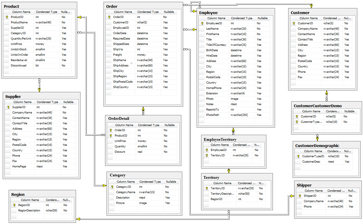
cur = sqlite3.Cursor(conn)

cur.execute('''SELECT name 
               FROM sqlite_master
               WHERE type='table';''')

df_table = pd.DataFrame(cur.fetchall(), columns=['Table'])

df_table # Verifying the images results

.dataframe tbody tr th {
    vertical-align: top;
}

.dataframe thead th {
    text-align: right;
}

</style>

	Table
0	Employee
1	Category
2	Customer
3	Shipper
4	Supplier
5	Order
6	Product
7	OrderDetail
8	CustomerCustomerDemo
9	CustomerDemographic
10	Region
11	Territory
12	EmployeeTerritory

Q1: Does discount amount have a statistically significant effect on the quantity of a product in an order? If so, at what level(s) of discount?

$H_0$: Discount amount does not significantly effect the amount of products ordered.
$H_1$: Discounts do have a significant effect (positive or negative) on the amount of products ordered.

For this test, I will be using a two-tailed test.

Initial Query & Feature Engineering

cur.execute('''SELECT *
               FROM OrderDetail o;''')
df1 = pd.DataFrame(cur.fetchall()) 
df1.columns = [i[0] for i in cur.description]
df1.head()

.dataframe tbody tr th {
    vertical-align: top;
}

.dataframe thead th {
    text-align: right;
}

</style>

	Id	OrderId	ProductId	UnitPrice	Quantity
0	10248/11	10248	11	14.0	12
1	10248/42	10248	42	9.8	10
2	10248/72	10248	72	34.8	5
3	10249/14	10249	14	18.6	9
4	10249/51	10249	51	42.4	40

Here I look to create a boolean column to indicated if a column has been discounted or not.

df1['Discounted'] = df1['Discount'] > 0

df1['Discounted'].sum() # How many discounted (True) orders are there?

df1.head() # Quick check

.dataframe tbody tr th {
    vertical-align: top;
}

.dataframe thead th {
    text-align: right;
}

</style>

	Id	OrderId	ProductId	UnitPrice	Quantity	Discounted
0	10248/11	10248	11	14.0	12	False
1	10248/42	10248	42	9.8	10	False
2	10248/72	10248	72	34.8	5	False
3	10249/14	10249	14	18.6	9	False
4	10249/51	10249	51	42.4	40	False

EDA

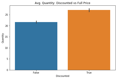
Checking to see whether or not there is a visual difference between the two groups: Discounted (True) or Full Price (False)

fig, ax = plt.subplots(figsize=(8,5))

sns.barplot(data=df1, x='Discounted', y='Quantity', ci=68, ax=ax)
sns.set(style='darkgrid')
plt.title('Avg. Quantity: Discounted vs Full Price');

In order to have a more flexible instance of my target data, I need to move the information from the DataFrame into a python dictionary.

quantVSdisc = {}
for item in df1['Discounted'].unique():
    quantVSdisc[item] = df1.groupby('Discounted').get_group(item)['Quantity']

print(len(quantVSdisc[False]), len(quantVSdisc[True])) 
# Confirming results transferred to dictionary

1317 838

It is clear, visually, that there may be a valid effect on the quantity purchased if the order is discounted. There are two groups of interest and thus I will be checking the assumptions for a 2 Sample T-test.

Testing Assumptions (2 Sample T-test)

Outliers?

fig, ax = plt.subplots(figsize=(8,5))

for key, val in quantVSdisc.items():
    if key == True:
        lab = 'Discounted'
    else:
        lab = 'Full Price'
        
    sns.distplot(val, label=key, ax=ax)

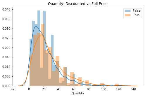
plt.title('Quantity: Discounted vs Full Price')
ax.legend();

# Visual check for skew

Although skewed, the tails do not look very thick, will remove some outliers to try for better normality since I have a lot of data still.

for key, val in quantVSdisc.items():
    out_dict = fn.find_outliers_Z(val)
    print(f'There are {out_dict.sum()} {key} Z-outliers.')
    
    out_dict = fn.find_outliers_IQR(val)
    print(f'There are {out_dict.sum()} {key} IQR-outliers.')

There are 20 False Z-outliers.
There are 34 False IQR-outliers.
There are 15 True Z-outliers.
There are 29 True IQR-outliers.

Checking IQR method for posterity, although I intend to use the Z-score method to remain conservative with removal of data.

for key, val in quantVSdisc.items():
    out_dict = fn.find_outliers_Z(val)
    quantVSdisc[key] = val[~out_dict]
    
# Removing values outside of +/- 3 Z-scores from mean directly from dictionary

fig, ax = plt.subplots(figsize=(8,5))

for key, val in quantVSdisc.items():
    if key == True:
        lab = 'Discounted'
    else:
        lab = 'Full Price'
        
    sns.distplot(val, label=lab, ax=ax)

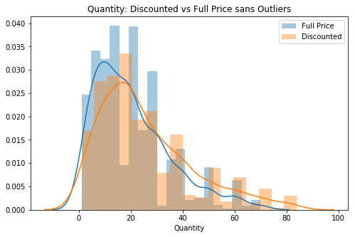
plt.title('Quantity: Discounted vs Full Price sans Outliers')
ax.legend();

# 2nd visual check (now without outliers)

The data looks a lot closer to standard normal. Now I can move forward to test normality.

Normality?

for key, val in quantVSdisc.items():
    stat, p = stats.normaltest(val)
    
    if key == True:
        lab = 'Discounted'
    else:
        lab = 'Full Price'
    
    print(f'{lab} normal test p-value = {round(p,4)}')
    
    sig = 'is NOT' if p < .05 else 'IS'
    
    print(f'The data {sig} normal.')

Full Price normal test p-value = 0.0
The data is NOT normal.
Discounted normal test p-value = 0.0
The data is NOT normal.

print(len(quantVSdisc[False]), len(quantVSdisc[True]))

1297 823

The data is not normal in either sample. This means to move forward I need to have samples larger than 15 each (recommended). Since I have 1,297 Full Price and 823 Discounted I can do so.

Equal Variance?

In order for stats.levene() to properly accept my data, I need to unpack my dictionary into a list.

norm_list = []

for key, val in quantVSdisc.items():
    norm_list.append(val)

stat, p = stats.levene(*norm_list)

print(f'Levene test p-value = {round(p,4)}')

sig = 'does NOT' if p < .05 else 'DOES'

print(f'The data {sig} have equal variance.')

Levene test p-value = 0.0
The data does NOT have equal variance.

Since the Levene test was failed, I must use the Welch's T-test function with the 'equal_var' parameter set to 'False' in order to determine whether or not I am dealing with two samples from different populations and test my hypothesis.

Hypothesis Test

stat, p = stats.ttest_ind(*norm_list, equal_var=False)

print(f"Welch's T-test p-value = {round(p,4)}")

sig = 'IS' if p < .05 else 'is NOT'

print(f'The data {sig} from different populations.')

Welch's T-test p-value = 0.0
The data IS from different populations.

The data does NOT have equal variance but IS from different populations. Given the information above, I can move forward with Rejecting the Null Hypothesis ($H_0$).

Post-Hoc Calculations

eff_size = fn.Cohen_d(quantVSdisc[True], quantVSdisc[False])

eff_size

0.32001140965727837

Given the standard interpretation of Cohen's D, our value falls between the 'small effect' category (0.2) and 'medium effect' category (0.5). Therefore we can say, although relatively small, discounts do have an effect on the quantity purchased.

model = pairwise_tukeyhsd(df1['Quantity'], df1['Discount'])
model.summary()

Multiple Comparison of Means - Tukey HSD,FWER=0.05

group1	group2	meandiff	lower	upper	reject
0.0	0.01	-19.7153	-80.3306	40.9001	False
0.0	0.02	-19.7153	-62.593	23.1625	False
0.0	0.03	-20.0486	-55.0714	14.9742	False
0.0	0.04	-20.7153	-81.3306	39.9001	False
0.0	0.05	6.2955	1.5381	11.053	True
0.0	0.06	-19.7153	-80.3306	40.9001	False
0.0	0.1	3.5217	-1.3783	8.4217	False
0.0	0.15	6.6669	1.551	11.7828	True
0.0	0.2	5.3096	0.2508	10.3684	True
0.0	0.25	6.525	1.3647	11.6852	True
0.01	0.02	0.0	-74.2101	74.2101	False
0.01	0.03	-0.3333	-70.2993	69.6326	False
0.01	0.04	-1.0	-86.6905	84.6905	False
0.01	0.05	26.0108	-34.745	86.7667	False
0.01	0.06	0.0	-85.6905	85.6905	False
0.01	0.1	23.237	-37.5302	84.0042	False
0.01	0.15	26.3822	-34.4028	87.1671	False
0.01	0.2	25.0248	-35.7554	85.805	False
0.01	0.25	26.2403	-34.5485	87.029	False
0.02	0.03	-0.3333	-55.6463	54.9796	False
0.02	0.04	-1.0	-75.2101	73.2101	False
0.02	0.05	26.0108	-17.0654	69.087	False
0.02	0.06	0.0	-74.2101	74.2101	False
0.02	0.1	23.237	-19.8552	66.3292	False
0.02	0.15	26.3822	-16.7351	69.4994	False
0.02	0.2	25.0248	-18.0857	68.1354	False
0.02	0.25	26.2403	-16.8823	69.3628	False
0.03	0.04	-0.6667	-70.6326	69.2993	False
0.03	0.05	26.3441	-8.9214	61.6096	False
0.03	0.06	0.3333	-69.6326	70.2993	False
0.03	0.1	23.5703	-11.7147	58.8553	False
0.03	0.15	26.7155	-8.6001	62.0311	False
0.03	0.2	25.3582	-9.9492	60.6656	False
0.03	0.25	26.5736	-8.7485	61.8957	False
0.04	0.05	27.0108	-33.745	87.7667	False
0.04	0.06	1.0	-84.6905	86.6905	False
0.04	0.1	24.237	-36.5302	85.0042	False
0.04	0.15	27.3822	-33.4028	88.1671	False
0.04	0.2	26.0248	-34.7554	86.805	False
0.04	0.25	27.2403	-33.5485	88.029	False
0.05	0.06	-26.0108	-86.7667	34.745	False
0.05	0.1	-2.7738	-9.1822	3.6346	False
0.05	0.15	0.3714	-6.2036	6.9463	False
0.05	0.2	-0.986	-7.5166	5.5447	False
0.05	0.25	0.2294	-6.3801	6.839	False
0.06	0.1	23.237	-37.5302	84.0042	False
0.06	0.15	26.3822	-34.4028	87.1671	False
0.06	0.2	25.0248	-35.7554	85.805	False
0.06	0.25	26.2403	-34.5485	87.029	False
0.1	0.15	3.1452	-3.5337	9.824	False
0.1	0.2	1.7879	-4.8474	8.4231	False
0.1	0.25	3.0033	-3.7096	9.7161	False
0.15	0.2	-1.3573	-8.1536	5.4389	False
0.15	0.25	-0.1419	-7.014	6.7302	False
0.2	0.25	1.2154	-5.6143	8.0451	False

Given an alpha level of 0.05, I can reject the null hypothesis for the following discount levels:

Q1 Summary

After testing my hypothesis regarding quantity on discounted orders, I can say to stakeholders that discounting does in fact have, with 95% confidence, an effect on the quantity of any given order.

Additionally, I can say that the discount levels (in descending order) of 15%, 25%, 5%, 20% have the most significant effect on the avg. quantity of a given order.

Q2: Does discount amount have a statistically significant effect on the total amount spent in an order? If so, at what level(s) of discount?

$H_0$: Discount amount does not significantly effect the total amount of money spent.
$H_1$: Discounts do have a significant effect (positive or negative) on the total amount of money spent.

For this test, I will be using a two-tailed test.

Initial Query & Feature Engineering

I will do a very similar setup to the previous hypothesis for the quantity exploration.

cur.execute('''SELECT *
               FROM OrderDetail o;''')
df2 = pd.DataFrame(cur.fetchall()) 
df2.columns = [i[0] for i in cur.description]
df2.head()

.dataframe tbody tr th {
    vertical-align: top;
}

.dataframe thead th {
    text-align: right;
}

</style>

	Id	OrderId	ProductId	UnitPrice	Quantity
0	10248/11	10248	11	14.0	12
1	10248/42	10248	42	9.8	10
2	10248/72	10248	72	34.8	5
3	10249/14	10249	14	18.6	9
4	10249/51	10249	51	42.4	40

df2['Discounted'] = df2['Discount'] > 0
# Creating boolean column for discount or full price

df2['TotalSpent'] = (df2['UnitPrice'] * (1-df2['Discount'])) * df2['Quantity']
# Creating a numerical column for total price spent per order (including discount)

df2.head() # Quick check

.dataframe tbody tr th {
    vertical-align: top;
}

.dataframe thead th {
    text-align: right;
}

</style>

	Id	OrderId	ProductId	UnitPrice	Quantity	Discounted	TotalSpent
0	10248/11	10248	11	14.0	12	False	168.0
1	10248/42	10248	42	9.8	10	False	98.0
2	10248/72	10248	72	34.8	5	False	174.0
3	10249/14	10249	14	18.6	9	False	167.4
4	10249/51	10249	51	42.4	40	False	1696.0

EDA

# Visual check

fig, ax = plt.subplots(figsize=(8,5))

sns.barplot(data=df2, x='Discounted', y='TotalSpent', ci=68, ax=ax)
sns.set(style='darkgrid')
plt.title('Avg. TotalSpent: Discounted vs Full Price');

Converting to a dictionary for flexibility (as before)

totspentVSdisc = {}
for item in df2['Discounted'].unique():
    totspentVSdisc[item] = df2.groupby('Discounted').get_group(item)['TotalSpent']

print(len(totspentVSdisc[False]), len(totspentVSdisc[True]))
# Verifying results

1317 838

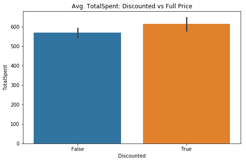
There is, once again visually, a small difference in the average total spent per order. Not too hopeful of its significance, but it is still worth investigation. As with my first hypothesis, this will fall under a 2 Sample T-test.

Testing Assumptions (2 Sample T-test)

Outliers?

fig, ax = plt.subplots(figsize=(8,5))

for key, val in totspentVSdisc.items():
    if key == True:
        lab = 'Discounted'
    else:
        lab = 'Full Price'
        
    sns.distplot(val, label=key, ax=ax)

plt.title('Total Spent: Discounted vs Full Price')
ax.legend();

# Visual check for skew

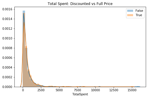
This is highly skewed to the right, although very thin.

for key, val in totspentVSdisc.items():
    out_dict = fn.find_outliers_Z(val)
    print(f'There are {out_dict.sum()} {key} Z-outliers.')
    
    out_dict = fn.find_outliers_IQR(val)
    print(f'There are {out_dict.sum()} {key} IQR-outliers.')

There are 19 False Z-outliers.
There are 101 False IQR-outliers.
There are 16 True Z-outliers.
There are 66 True IQR-outliers.

Despite there being a very long tail, I will for consistency stick with Z-scores in order to remain conservative.

for key, val in totspentVSdisc.items():
    out_dict = fn.find_outliers_Z(val)
    totspentVSdisc[key] = val[~out_dict]
    
# Removing values outside of +/- 3 Z-scores from mean directly from dictionary

fig, ax = plt.subplots(figsize=(8,5))

for key, val in totspentVSdisc.items():
    if key == True:
        lab = 'Discounted'
    else:
        lab = 'Full Price'
        
    sns.distplot(val, label=lab, ax=ax)

plt.title('Total Spent: Discounted vs Full Price sans Outliers')
ax.legend();

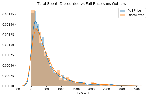
# 2nd visual check (now without outliers)

Although, if compared to the standard normal distribution, the data is still pretty skewed to the right. I will move forward with testing assumptions.

Normality?

for key, val in totspentVSdisc.items():
    stat, p = stats.normaltest(val)
    
    if key == True:
        lab = 'Discounted'
    else:
        lab = 'Full Price'
    
    print(f'{lab} normal test p-value = {round(p,4)}')
    
    sig = 'is NOT' if p < .05 else 'IS'
    
    print(f'The data {sig} normal.')

Full Price normal test p-value = 0.0
The data is NOT normal.
Discounted normal test p-value = 0.0
The data is NOT normal.

No surprises here, this data is not normal.

print(len(totspentVSdisc[False]), len(totspentVSdisc[True]))

1298 822

Luckily, with Full Price group having 1,298 and Discounted having 822, I am able to ignore the need for normality and move on to check for equal variance.

Equal Variance?

# Same as before

norm_list2 = []

for key, val in totspentVSdisc.items():
    norm_list2.append(val)

stat, p = stats.levene(*norm_list2)

print(f'Levene test p-value = {round(p,4)}')

sig = 'does NOT' if p < .05 else 'DOES'

print(f'The data {sig} have equal variance.')

Levene test p-value = 0.4614
The data DOES have equal variance.

Since the data does pass all of the assumption tests, I can move forward with a normal 2 Sample T-test.

Hypothesis Test

stat, p = stats.ttest_ind(*norm_list2)

print(f"Welch's T-test p-value = {round(p,4)}")

sig = 'IS' if p < .05 else 'is NOT'

print(f'The data {sig} from different populations.')

Welch's T-test p-value = 0.2057
The data is NOT from different populations.

At this point, I have failed to reject the null hypothesis.

Post-Hoc Calculations

Although I have failed to reject the null, I want to investigate if at a given level, a discount does have a significant effect upon the total amount spent.

model2 = pairwise_tukeyhsd(df2['TotalSpent'], df2['Discount'])
model2.summary()

Multiple Comparison of Means - Tukey HSD,FWER=0.05

group1	group2	meandiff	lower	upper	reject
0.0	0.01	-540.3065	-3662.2549	2581.6418	False
0.0	0.02	-540.1165	-2748.5047	1668.2716	False
0.0	0.03	-529.703	-2333.5278	1274.1217	False
0.0	0.04	-492.2465	-3614.1949	2629.7018	False
0.0	0.05	227.9252	-17.1036	472.954	False
0.0	0.06	-506.0865	-3628.0349	2615.8618	False
0.0	0.1	-41.1098	-293.48	211.2604	False
0.0	0.15	-12.6424	-276.1341	250.8493	False
0.0	0.2	-16.0866	-276.6374	244.4641	False
0.0	0.25	72.4517	-193.3232	338.2266	False
0.01	0.02	0.19	-3821.9494	3822.3294	False
0.01	0.03	10.6035	-3592.9441	3614.1511	False
0.01	0.04	48.06	-4365.3664	4461.4864	False
0.01	0.05	768.2318	-2360.9551	3897.4187	False
0.01	0.06	34.22	-4379.2064	4447.6464	False
0.01	0.1	499.1968	-2630.5736	3628.9671	False
0.01	0.15	527.6642	-2603.0226	3658.3509	False
0.01	0.2	524.2199	-2606.2207	3654.6605	False
0.01	0.25	612.7582	-2518.1215	3743.638	False
0.02	0.03	10.4135	-2838.441	2859.268	False
0.02	0.04	47.87	-3774.2694	3870.0094	False
0.02	0.05	768.0418	-1450.5676	2986.6511	False
0.02	0.06	34.03	-3788.1094	3856.1694	False
0.02	0.1	499.0068	-1720.4254	2718.4389	False
0.02	0.15	527.4742	-1693.2501	2748.1984	False
0.02	0.2	524.0299	-1696.3473	2744.4071	False
0.02	0.25	612.5682	-1608.4281	2833.5645	False
0.03	0.04	37.4565	-3566.0911	3641.0041	False
0.03	0.05	757.6283	-1058.6958	2573.9523	False
0.03	0.06	23.6165	-3579.9311	3627.1641	False
0.03	0.1	488.5933	-1328.7357	2305.9222	False
0.03	0.15	517.0607	-1301.8461	2335.9674	False
0.03	0.2	513.6164	-1304.8666	2332.0994	False
0.03	0.25	602.1547	-1217.0842	2421.3936	False
0.04	0.05	720.1718	-2409.0151	3849.3587	False
0.04	0.06	-13.84	-4427.2664	4399.5864	False
0.04	0.1	451.1368	-2678.6336	3580.9071	False
0.04	0.15	479.6042	-2651.0826	3610.2909	False
0.04	0.2	476.1599	-2654.2807	3606.6005	False
0.04	0.25	564.6982	-2566.1815	3695.578	False
0.05	0.06	-734.0118	-3863.1987	2395.1751	False
0.05	0.1	-269.035	-599.0955	61.0255	False
0.05	0.15	-240.5676	-579.2076	98.0724	False
0.05	0.2	-244.0119	-580.3686	92.3449	False
0.05	0.25	-155.4735	-495.8931	184.946	False
0.06	0.1	464.9768	-2664.7936	3594.7471	False
0.06	0.15	493.4442	-2637.2426	3624.1309	False
0.06	0.2	489.9999	-2640.4407	3620.4405	False
0.06	0.25	578.5382	-2552.3415	3709.418	False
0.1	0.15	28.4674	-315.5219	372.4568	False
0.1	0.2	25.0231	-316.7187	366.765	False
0.1	0.25	113.5615	-232.1799	459.3029	False
0.15	0.2	-3.4443	-353.4794	346.5909	False
0.15	0.25	85.0941	-268.847	439.0351	False
0.2	0.25	88.5383	-263.2188	440.2954	False

Q2 Summary

After testing my hypothesis regarding the total amount spent on discounted orders, I can say to stakeholders that discounting does not have, with 95% confidence, an effect on the total amount spent on any given order.

Additionally, I can say that no matter the discount level, there is no significant effect on the avg. amount spent on a given order.

Q3: Does the region in which the products are sold have a significant effect on the quantity of a product in an order? If so, which region buys the most?

$H_0$: RegionID does not significantly effect the amount of products ordered.
$H_1$: RegionID does have a significant effect (positive or negative) on the amount of products ordered.

For this test, I will be using a two-tailed test.

Initial Query & Feature Engineering

cur.execute('''SELECT DISTINCT(o.OrderId), o.Quantity, r.Id, r.RegionDescription
               FROM OrderDetail o
               JOIN 'Order' ord
               ON o.OrderId = ord.Id
               JOIN Employee e
               ON ord.EmployeeId = e.Id
               JOIN EmployeeTerritory et
               USING(EmployeeId)
               JOIN Territory t
               ON et.TerritoryId = t.Id
               JOIN Region r
               ON r.Id = t.RegionId;''') 
df3 = pd.DataFrame(cur.fetchall()) 
df3.columns = [i[0] for i in cur.description]
df3.head()

.dataframe tbody tr th {
    vertical-align: top;
}

.dataframe thead th {
    text-align: right;
}

</style>

	OrderId	Quantity	Id	RegionDescription
0	10248	12	1	Eastern
1	10248	10	1	Eastern
2	10248	5	1	Eastern
3	10249	9	2	Western
4	10249	40	2	Western

I ran into a duplication error due to (likely) the Order Id and Employee Id's being one-to-many during the joining process; coercing the OrderIds to be distinct should solve this.

EDA

Region Descriptors

'Eastern'
'Western'
'Northern'
'Southern'

fig, ax = plt.subplots(figsize=(8,5))

sns.barplot(data=df3, x='RegionDescription', y='Quantity', ci=68, ax=ax)

plt.title('Avg. Quantity: By Region');

# Quick check of differences via swarmplot

#fig, ax = plt.subplots(figsize=(8,5))

sns.catplot(data=df3, x='RegionDescription', y='Quantity', kind='swarm', ci=68)

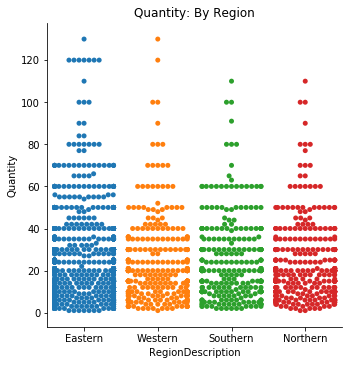
plt.title('Quantity: By Region');

quantVSreg = {}
for item in df3['RegionDescription'].unique():
    quantVSreg[item] = df3.groupby('RegionDescription').get_group(item)['Quantity']

for item in df3['RegionDescription'].unique():
    print(f'Number of instances in {item}: {len(quantVSreg[item])}')

Number of instances in Eastern: 1022
Number of instances in Western: 325
Number of instances in Southern: 302
Number of instances in Northern: 349

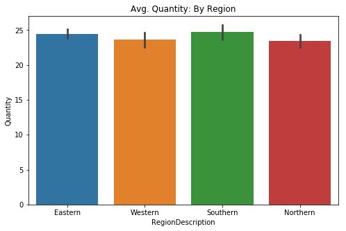
Visually there is not a large difference between regions, however my goal is simply to find out whether or not an effect exists. It is clear that the Eastern region does make up almost 50% of the orders they received during the period of time this data represents. Due to our data being more than two groups, I will need to proceed with a One-Way ANOVA test.

Testing Assumptions (One-Way ANOVA)

Outliers?

fig, ax = plt.subplots(figsize=(8,5))

for key, val in quantVSreg.items():       
    sns.distplot(val, label=key, ax=ax)

plt.title('Quantity: by Region')
ax.legend();

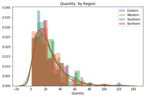
# Visual check for skew

All of the groups appear to have a similar level of skew and weight in the right tail. There is one item for the Eastern group that hangs pretty far into the tail, I am interested to see whether or not it will fall off after outliers are removed.

for key, val in quantVSreg.items():
    out_dict = fn.find_outliers_Z(val)
    print(f'There are {out_dict.sum()} {key} Z-outliers.')
    
    #out_dict = fn.find_outliers_IQR(val)
    #print(f'There are {out_dict.sum()} {key} IQR-outliers.')

There are 14 Eastern Z-outliers.
There are 5 Western Z-outliers.
There are 4 Southern Z-outliers.
There are 8 Northern Z-outliers.

# Removing outliers per the Z-score method

for key, val in quantVSreg.items():
    out_dict = fn.find_outliers_Z(val)
    quantVSreg[key] = val[~out_dict]

fig, ax = plt.subplots(figsize=(8,5))

for key, val in quantVSreg.items():
    sns.distplot(val, label=key, ax=ax)

plt.title('Quantity: by Region sans Outliers')
ax.legend();

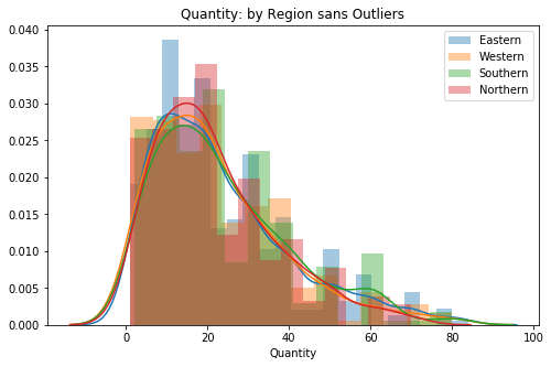
# 2nd visual check (now without outliers)

My function removed a large bit of the tails, and visually I can see that the Northern/Eastern groups do not skew out as far as the other two groups.

Normality?

for key, val in quantVSreg.items():
    stat, p = stats.normaltest(val)
        
    print(f'{key} normal test p-value = {round(p,4)}')
    
    sig = 'is NOT' if p < .05 else 'IS'
    
    print(f'The data {sig} normal.')

Eastern normal test p-value = 0.0
The data is NOT normal.
Western normal test p-value = 0.0
The data is NOT normal.
Southern normal test p-value = 0.0
The data is NOT normal.
Northern normal test p-value = 0.0
The data is NOT normal.

for item in df3['RegionDescription'].unique():
    print(f'Number of instances in {item}: {len(quantVSreg[item])}')

Number of instances in Eastern: 1008
Number of instances in Western: 320
Number of instances in Southern: 298
Number of instances in Northern: 341

Not a single group is considered normal. However, due to the groups all having more than 15 instances (by far), I am able to ignore this assumption and test for equal variance.

Equal Variance?

norm_list3 = []

for key, val in quantVSreg.items():
    norm_list3.append(val)

stat, p = stats.levene(*norm_list3)

print(f'Levene test p-value = {round(p,4)}')

sig = 'does NOT' if p < .05 else 'DOES'

print(f'The data {sig} have equal variance.')

Levene test p-value = 0.11
The data DOES have equal variance.

Since the data passed Levene's test, I am able to safely move forward with a standard One-Way ANOVA in order to see if my samples are from different populations and test my hypothesis.

Hypothesis Test

stat, p = stats.f_oneway(*norm_list3)

print(f"One-Way ANOVA p-value = {round(p,4)}")

sig = 'IS' if p < .05 else 'is NOT'

print(f'The data {sig} from different populations.')

One-Way ANOVA p-value = 0.3789
The data is NOT from different populations.

The data does NOT have a p-value low enought to say confidently that it is from different populations. Given the information above, I have failed to reject the Null Hypothesis ($H_0$).

Post-Hoc Calculations

Although I have failed to reject the null, (as with Q2) I want to investigate if inter-regionally, there is have a significant effect upon the average quantity ordered.

model3 = pairwise_tukeyhsd(df3['Quantity'], df3['RegionDescription'])
model3.summary()

Multiple Comparison of Means - Tukey HSD,FWER=0.05

group1	group2	meandiff	lower	upper	reject
Eastern	Northern	-1.0508	-4.1218	2.0202	False
Eastern	Southern	0.2852	-2.959	3.5295	False
Eastern	Western	-0.8925	-4.0468	2.2619	False
Northern	Southern	1.336	-2.5569	5.2289	False
Northern	Western	0.1583	-3.66	3.9766	False
Southern	Western	-1.1777	-5.1367	2.7813	False

Q3 Summary

After testing my hypothesis regarding the average quantity ordered per region, I can say to stakeholders that there is not, with 95% confidence, an effect on the average quantity purchased in a given order.

Additionally, I can say that between individual regions, there is no evidence to suggest a significant difference in the average quantity purchased in a given order.

Q4: Does whether the company keeps an item 'in stock' or not have any effect on the total spent on those products? If so, is there an optimal level to reorder?

$H_0$: The level at which Northwind re-orders products has no effect on the total amount spent on orders including those items.
$H_1$: Whether or not Northwind waits until they are out of stock to reorder has an effect on the total amount spent on orders with those items.

For this test, I will be using a two-tailed test.

Initial Query & Feature Engineering

cur.execute('''SELECT ord.ProductId, ord.Quantity, ord.UnitPrice, 
               ord.Discount, p.ReorderLevel, p.CategoryId, 
               ((ord.Quantity * ord.UnitPrice)*(1 - ord.Discount)) 
               AS TotalSpent
               FROM OrderDetail ord
               JOIN Product p
               ON ord.ProductId = p.Id;''')
df4 = pd.DataFrame(cur.fetchall()) 
df4.columns = [i[0] for i in cur.description]
df4.head()

.dataframe tbody tr th {
    vertical-align: top;
}

.dataframe thead th {
    text-align: right;
}

</style>

	ProductId	Quantity	UnitPrice	ReorderLevel	CategoryId	TotalSpent
0	11	12	14.0	30	4	168.0
1	42	10	9.8	0	5	98.0
2	72	5	34.8	0	4	174.0
3	14	9	18.6	0	7	167.4
4	51	40	42.4	10	7	1696.0

df4.ReorderLevel.value_counts() # Quick check of samples

0     718
15    273
25    256
10    242
30    235
20    235
5     196
Name: ReorderLevel, dtype: int64

df4.CategoryId.value_counts() # Spread check among categories (for later)

1    404
4    366
3    334
8    330
2    216
5    196
6    173
7    136
Name: CategoryId, dtype: int64

EDA

Reorder Levels

0 - 30 at five unit intervals (0, 5, 10,...30)

fig, ax = plt.subplots(figsize=(8,5))

sns.barplot(data=df4, x='ReorderLevel', y='TotalSpent', ci=68, ax=ax)

plt.title('Avg. TotalSpent: By ReorderLevel');

# Quick check of differences via swarmplot (like above)

#fig, ax = plt.subplots(figsize=(8,5))

sns.catplot(data=df4, x='ReorderLevel', y='TotalSpent', kind='swarm', ci=68)

plt.title('TotalSpent: By ReorderLevel');

totspentVSreord = {}
for item in df4['ReorderLevel'].unique():
    totspentVSreord[item] = df4.groupby('ReorderLevel').get_group(item)['TotalSpent']

# Quick check for correct data transfer

for item in sorted(df4['ReorderLevel'].unique()):
    print(f'Number of instances in {item}: {len(totspentVSreord[item])}')
    
# We're good!

Number of instances in 0: 718
Number of instances in 5: 196
Number of instances in 10: 242
Number of instances in 15: 273
Number of instances in 20: 235
Number of instances in 25: 256
Number of instances in 30: 235

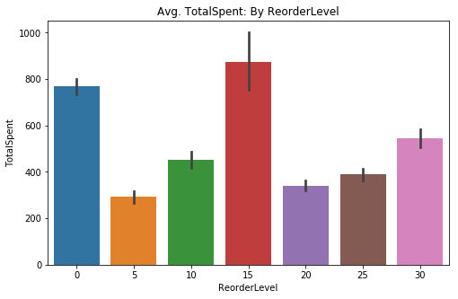
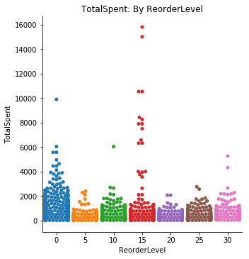
Visually, I can see that those at a 0 and 15 reorder level tend to stick out with the bar chart. The swarm chart demonstrates why the error bar is so large on the bar chart, the 15 unit reorder level seems to have a wide range of values. I will need to use the One-Way ANOVA test since I will be comparing multiple sample populations.

Testing Assumptions (One-Way ANOVA)

Outliers?

fig, ax = plt.subplots(figsize=(8,5))

for key, val in sorted(totspentVSreord.items()):       
    sns.distplot(val, label=key, ax=ax)

plt.title('TotalSpent: by Reorder Level')
ax.legend();

# Visual check for skew

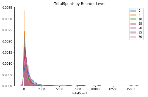
The extreme values in one or more of the reorder levels are skewing the distribution strongly. It seems best to remove them to ensure I get closer in the normality test.

for key, val in sorted(totspentVSreord.items()):
    out_dict = fn.find_outliers_Z(val)
    print(f'There are {out_dict.sum()} {key} Z-outliers.')
    
    #out_dict = fn.find_outliers_IQR(val)
    #print(f'There are {out_dict.sum()} {key} IQR-outliers.')
    
    #due to the number of categories, no need to check IQR

There are 15 0 Z-outliers.
There are 5 5 Z-outliers.
There are 3 10 Z-outliers.
There are 9 15 Z-outliers.
There are 5 20 Z-outliers.
There are 5 25 Z-outliers.
There are 3 30 Z-outliers.

Surprisingly, the 0 level has the most values outside of the +/- 3 z-score threshold.

# Removing outliers per the Z-score method

for key, val in totspentVSreord.items():
    out_dict = fn.find_outliers_Z(val)
    totspentVSreord[key] = val[~out_dict]

fig = plt.figure(figsize=(9,9))
ax1 = fig.add_subplot(211)
ax2 = fig.add_subplot(212, sharey=ax1)

helper = [0, 5, 10, 15]

for key, val in sorted(totspentVSreord.items()):
    if key in helper:
        sns.distplot(val, label=key, ax=ax1).set_title('Total Spent: by Reorder Level sans Outliers (0-15)')
        #plt.legend()
    else:
        sns.distplot(val, label=key, ax=ax2).set_title('Total Spent: by Reorder Level sans Outliers (20-30)')
        #plt.legend()
        
    ax1.legend()
    ax2.legend();
        
plt.tight_layout()


# 2nd visual check (now without outliers)

No handles with labels found to put in legend.
No handles with labels found to put in legend.
No handles with labels found to put in legend.
No handles with labels found to put in legend.

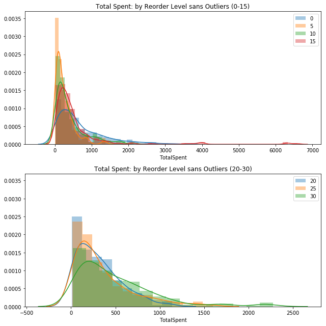
Visually it appears that there are some similarities between the groups I selected arbitrarily by numeric value. For the unit level of 5, there is a high amount that spikes around zero TotalSpent, while there is a long tail created by 15.

In the second plot, the categories reflect a similar relationship. Two of the categories have a large grouping around zero TotalSpent while the 30 reorder level creates a tail.

Normality?

for key, val in sorted(totspentVSreord.items()):
    stat, p = stats.normaltest(val)
        
    print(f'{key} normal test p-value = {round(p,4)}')
    
    sig = 'is NOT' if p < .05 else 'IS'
    
    print(f'The data {sig} normal.')

0 normal test p-value = 0.0
The data is NOT normal.
5 normal test p-value = 0.0
The data is NOT normal.
10 normal test p-value = 0.0
The data is NOT normal.
15 normal test p-value = 0.0
The data is NOT normal.
20 normal test p-value = 0.0
The data is NOT normal.
25 normal test p-value = 0.0
The data is NOT normal.
30 normal test p-value = 0.0
The data is NOT normal.

My visual observations were confirmed by stats.normaltest(). The data does not appear to be very close to the standard normal, but with the amount of observations in each group we can move forward here regardless of the failures.

# Quick check for sample sizes

for item in sorted(df4['ReorderLevel'].unique()):
    print(f'Number of instances in {item}: {len(totspentVSreord[item])}')

Number of instances in 0: 703
Number of instances in 5: 191
Number of instances in 10: 239
Number of instances in 15: 264
Number of instances in 20: 230
Number of instances in 25: 251
Number of instances in 30: 232

The requirement to proceed testing while failing normality is recommended at 15, so given these amounts, I will proceed.

Equal Variance?

norm_list4 = []

for key, val in sorted(totspentVSreord.items()):
    norm_list4.append(val)

stat, p = stats.levene(*norm_list4)

print(f'Levene test p-value = {round(p,4)}')

sig = 'does NOT' if p < .05 else 'DOES'

print(f'The data {sig} have equal variance.')

Levene test p-value = 0.0
The data does NOT have equal variance.

Hypothesis Test

stat, p = stats.f_oneway(*norm_list4)

print(f"One-Way ANOVA p-value = {round(p,4)}")

sig = 'IS' if p < .05 else 'is NOT'

print(f'The data {sig} from different populations.')

One-Way ANOVA p-value = 0.0
The data IS from different populations.

It turns out, despite failing all of the assumptions, we were able to generate a p-value low enough to Reject the Null Hypothesis ($H_0$).

Post-Hoc Calculations

model4 = pairwise_tukeyhsd(df4['TotalSpent'], df4['ReorderLevel'])
model4.summary()

Multiple Comparison of Means - Tukey HSD,FWER=0.05

group1	group2	meandiff	lower	upper	reject
0	5	-477.8568	-703.3779	-252.3357	True
0	10	-316.1781	-524.1813	-108.1749	True
0	15	102.942	-96.0326	301.9165	False
0	20	-428.3497	-638.6571	-218.0423	True
0	25	-378.7012	-582.4062	-174.9963	True
0	30	-223.5092	-433.8166	-13.2018	True
5	10	161.6786	-107.2305	430.5878	False
5	15	580.7987	318.8108	842.7867	True
5	20	49.5071	-221.1884	320.2025	False
5	25	99.1556	-166.4429	364.754	False
5	30	254.3476	-16.3479	525.043	False
10	15	419.1201	172.0507	666.1895	True
10	20	-112.1716	-368.4558	144.1127	False
10	25	-62.5231	-313.4177	188.3715	False
10	30	92.6689	-163.6153	348.9532	False
15	20	-531.2917	-780.304	-282.2793	True
15	25	-481.6432	-725.105	-238.1814	True
15	30	-326.4512	-575.4635	-77.4388	True
20	25	49.6485	-203.1597	302.4567	False
20	30	204.8405	-53.3174	462.9984	False
25	30	155.192	-97.6162	408.0002	False

Significant results:

0 reorder level was shown to be different from all levels except 15
15 reorder level was shown to be different from all other levels
No other reorder level proved to be different from each other

Given this knowledge I will look a bit further into these two areas and see if there is anything worthwhile.

Q4 Summary

Given we know that there is an actual difference in the total revenue generated by products at the 15 unit threshold and those that are not reordered until stock is out (0), we can then look to how and why the data could be this way.

For example, the reason that those products at the 'sold out' threshold may be items ordered less often, in smaller batches, but have a higher average price. Similarly, those items at the 15 unit threshold may be this company's 'staple' products and thus are required to be on hand in a moderate capacity. This information alone can help inform the stakeholders on how to structure their reorder process to reduce waste.

Q5: Does the sales representative making the deal have a significant effect on the amount of product ordered? How about total spent?

$H_0$: The sales person brokering the deal does not have a significant effect on the amount of product in an order nor the total spent.
$H_1$: The sales person brokering the deal does have a significant effect on the amount of product in an order nor the total spent.

For this test, I will be using a two-tailed test.

Initial Query & Feature Engineering

cur.execute('''SELECT od.UnitPrice, od.Quantity, od.Discount,
               ((od.Quantity * od.UnitPrice)*(1 - od.Discount))
               AS TotalSpent, e.Id AS EmployeeId, e.LastName, e.FirstName, e.Title
               FROM OrderDetail od
               JOIN 'Order' o
               ON o.Id = od.OrderId
               JOIN Employee e
               ON o.EmployeeId = e.Id;''')
df5 = pd.DataFrame(cur.fetchall()) 
df5.columns = [i[0] for i in cur.description]
df5.head()

.dataframe tbody tr th {
    vertical-align: top;
}

.dataframe thead th {
    text-align: right;
}

</style>

	UnitPrice	Quantity	TotalSpent	EmployeeId	LastName	FirstName	Title
0	14.0	12	168.0	5	Buchanan	Steven	Sales Manager
1	9.8	10	98.0	5	Buchanan	Steven	Sales Manager
2	34.8	5	174.0	5	Buchanan	Steven	Sales Manager
3	18.6	9	167.4	6	Suyama	Michael	Sales Representative
4	42.4	40	1696.0	6	Suyama	Michael	Sales Representative

df5.shape

(2155, 8)

EDA

fig, ax = plt.subplots(figsize=(8,5))

sns.barplot(data=df5, x='EmployeeId', y='Quantity', ci=68, ax=ax)

plt.title('Avg. Quantity: By Salesperson');

sns.catplot(data=df5, x='EmployeeId', y='Quantity', kind='swarm', ci=68)

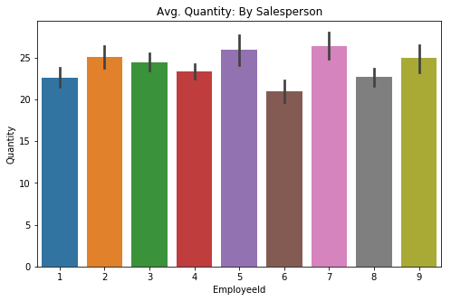
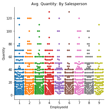
plt.title('Avg. Quantity: By Salesperson');

There appears to be some differences, albeit slight, for each employee in regards to quanity sold per order. The swarmplot shows what looks to be a fairly even distribution between each of the employees. The error bars in the barplot indicate that these differences may be 'give-or-take' around the same level.

fig, ax = plt.subplots(figsize=(8,5))

sns.barplot(data=df5, x='EmployeeId', y='TotalSpent', ci=68, ax=ax)

plt.title('Avg. TotalSpent: By Salesperson');

sns.catplot(data=df5, x='EmployeeId', y='TotalSpent', kind='swarm', ci=68)

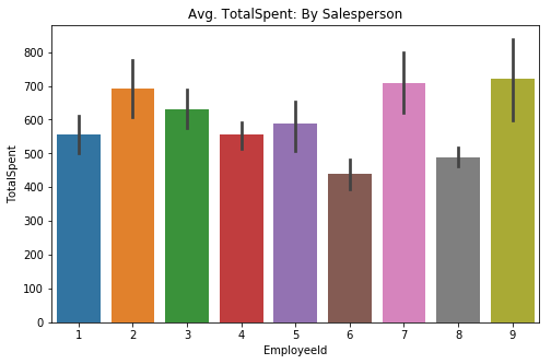
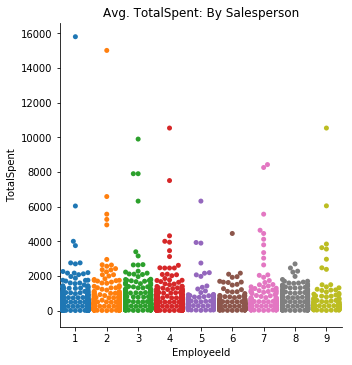
plt.title('Avg. TotalSpent: By Salesperson');

Visually speaking, the TotalSpent category show a lot more variation on the barplot between employees. The swarmplot however, tells a story that appears to indicate not much of a difference between the individual employees.

quantVSemp = {}
for item in df5['EmployeeId'].unique():
    quantVSemp[item] = df5.groupby('EmployeeId').get_group(item)['Quantity']

for item in sorted(df5['EmployeeId'].unique()):
    print(f'Number of instances in {item}: {len(quantVSemp[item])}')

Number of instances in 1: 345
Number of instances in 2: 241
Number of instances in 3: 321
Number of instances in 4: 420
Number of instances in 5: 117
Number of instances in 6: 168
Number of instances in 7: 176
Number of instances in 8: 260
Number of instances in 9: 107

totspentVSemp = {}
for item in df5['EmployeeId'].unique():
    totspentVSemp[item] = df5.groupby('EmployeeId').get_group(item)['TotalSpent']

for item in sorted(df5['EmployeeId'].unique()):
    print(f'Number of instances in {item}: {len(totspentVSemp[item])}')

Number of instances in 1: 345
Number of instances in 2: 241
Number of instances in 3: 321
Number of instances in 4: 420
Number of instances in 5: 117
Number of instances in 6: 168
Number of instances in 7: 176
Number of instances in 8: 260
Number of instances in 9: 107

Simply put, I will need to use a One-Way ANOVA test. This is due to the fact I have nine different employees (categories) that I will need to evaluate against each other.

Testing Assumptions (One-Way ANOVA)

Outliers?

fig, ax = plt.subplots(figsize=(8,5))

for key, val in sorted(quantVSemp.items()):       
    sns.distplot(val, label=key, ax=ax)

plt.title('Quantity: by Salesperson')
ax.legend();

# Check for overall skew of all data

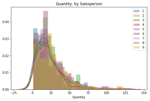
It appears that this data is fairly normal, I do not expect too many outliers to be pulled from the right tail.

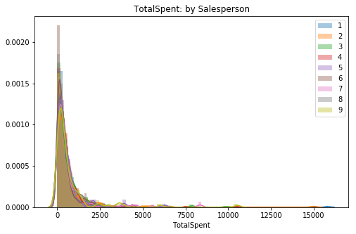
fig, ax = plt.subplots(figsize=(8,5))

for key, val in sorted(totspentVSemp.items()):       
    sns.distplot(val, label=key, ax=ax)

plt.title('TotalSpent: by Salesperson')
ax.legend();

This set appears to be way more skewed than the quantity data. I expect our outlier remove to cut a decent bit off of the right-side tail.

for key, val in sorted(quantVSemp.items()):
    out_dict = fn.find_outliers_Z(val)
    print(f'There are {out_dict.sum()} Z-outliers (quantity) for employee #{key}.')
    
    #out_dict = fn.find_outliers_IQR(val)
    #print(f'There are {out_dict.sum()} {key} IQR-outliers.')

There are 4 Z-outliers (quantity) for employee #1.
There are 4 Z-outliers (quantity) for employee #2.
There are 7 Z-outliers (quantity) for employee #3.
There are 5 Z-outliers (quantity) for employee #4.
There are 3 Z-outliers (quantity) for employee #5.
There are 2 Z-outliers (quantity) for employee #6.
There are 5 Z-outliers (quantity) for employee #7.
There are 6 Z-outliers (quantity) for employee #8.
There are 2 Z-outliers (quantity) for employee #9.

for key, val in sorted(totspentVSemp.items()):
    out_dict = fn.find_outliers_Z(val)
    print(f'There are {out_dict.sum()} Z-outliers (total spent) for employee #{key}.')
    
    #out_dict = fn.find_outliers_IQR(val)
    #print(f'There are {out_dict.sum()} {key} IQR-outliers.')

There are 4 Z-outliers (total spent) for employee #1.
There are 5 Z-outliers (total spent) for employee #2.
There are 4 Z-outliers (total spent) for employee #3.
There are 7 Z-outliers (total spent) for employee #4.
There are 3 Z-outliers (total spent) for employee #5.
There are 3 Z-outliers (total spent) for employee #6.
There are 5 Z-outliers (total spent) for employee #7.
There are 5 Z-outliers (total spent) for employee #8.
There are 2 Z-outliers (total spent) for employee #9.

I am surprised to see that the TotalSpent data had about the amount of outliers despite what the distplots show of it. Perhaps there are only a few data points dragging it out that far. I am interested to see what the data looks like after removal.

# Z-score method removal 

for key, val in quantVSemp.items():
    out_dict = fn.find_outliers_Z(val)
    quantVSemp[key] = val[~out_dict]

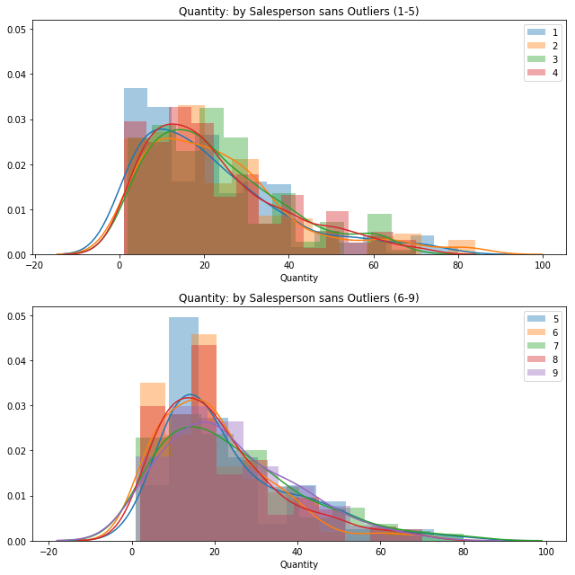
fig = plt.figure(figsize=(9,9))
ax1 = fig.add_subplot(211)
ax2 = fig.add_subplot(212, sharey=ax1)

helper2 = [1, 2, 3, 4]

for key, val in sorted(quantVSemp.items()):
    if key in helper2:
        sns.distplot(val, label=key, ax=ax1).set_title('Quantity: by Salesperson sans Outliers (1-5)')
    else:
        sns.distplot(val, label=key, ax=ax2).set_title('Quantity: by Salesperson sans Outliers (6-9)')
        
    ax1.legend()
    ax2.legend();
        
plt.tight_layout()

No handles with labels found to put in legend.
No handles with labels found to put in legend.
No handles with labels found to put in legend.
No handles with labels found to put in legend.

Looking at these graphs, it appears that employees 5, 6, and 8 have a higher percentage of their orders being quantities less than 20. Otherwise both groups seem to be about the same.

for key, val in totspentVSemp.items():
    out_dict = fn.find_outliers_Z(val)
    totspentVSemp[key] = val[~out_dict]

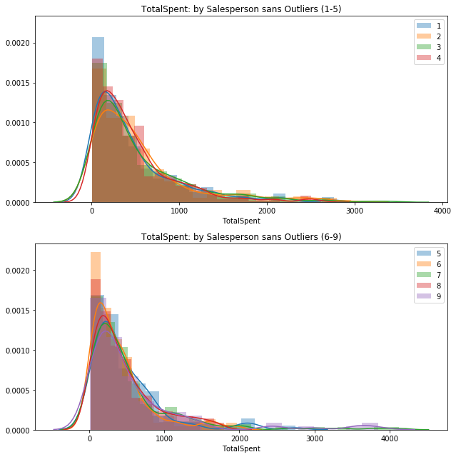
fig = plt.figure(figsize=(9,9))
ax1 = fig.add_subplot(211)
ax2 = fig.add_subplot(212, sharey=ax1)

helper2 = [1, 2, 3, 4]

for key, val in sorted(totspentVSemp.items()):
    if key in helper2:
        sns.distplot(val, label=key, ax=ax1).set_title('TotalSpent: by Salesperson sans Outliers (1-5)')
    else:
        sns.distplot(val, label=key, ax=ax2).set_title('TotalSpent: by Salesperson sans Outliers (6-9)')
        
    ax1.legend()
    ax2.legend();
        
plt.tight_layout()

No handles with labels found to put in legend.
No handles with labels found to put in legend.
No handles with labels found to put in legend.
No handles with labels found to put in legend.

Visually, these two groups appear to be quite similar. The second group just has a bit longer of a right-tail due to a few instances.

Normality?

for key, val in sorted(quantVSemp.items()):
    stat, p = stats.normaltest(val)
        
    print(f'Employee #{key} normal test p-value = {round(p,4)}')
    
    sig = 'is NOT' if p < .05 else 'IS'
    
    print(f'The data {sig} normal.')

Employee #1 normal test p-value = 0.0
The data is NOT normal.
Employee #2 normal test p-value = 0.0
The data is NOT normal.
Employee #3 normal test p-value = 0.0
The data is NOT normal.
Employee #4 normal test p-value = 0.0
The data is NOT normal.
Employee #5 normal test p-value = 0.0
The data is NOT normal.
Employee #6 normal test p-value = 0.0
The data is NOT normal.
Employee #7 normal test p-value = 0.0
The data is NOT normal.
Employee #8 normal test p-value = 0.0
The data is NOT normal.
Employee #9 normal test p-value = 0.0115
The data is NOT normal.

Although it Employee #9 had a p-value slightly smaller than our alpha, all groups have been determined to be non-normal. I will double-check that we have large enough sample sizes to move forward.

for item in sorted(df5['EmployeeId'].unique()):
    print(f'Number of instances in Employee #{item}: {len(quantVSemp[item])}')

Number of instances in Employee #1: 341
Number of instances in Employee #2: 237
Number of instances in Employee #3: 314
Number of instances in Employee #4: 415
Number of instances in Employee #5: 114
Number of instances in Employee #6: 166
Number of instances in Employee #7: 171
Number of instances in Employee #8: 254
Number of instances in Employee #9: 105

for key, val in sorted(totspentVSemp.items()):
    stat, p = stats.normaltest(val)
        
    print(f'Employee #{key} normal test p-value = {round(p,4)}')
    
    sig = 'is NOT' if p < .05 else 'IS'
    
    print(f'The data {sig} normal.')

Employee #1 normal test p-value = 0.0
The data is NOT normal.
Employee #2 normal test p-value = 0.0
The data is NOT normal.
Employee #3 normal test p-value = 0.0
The data is NOT normal.
Employee #4 normal test p-value = 0.0
The data is NOT normal.
Employee #5 normal test p-value = 0.0
The data is NOT normal.
Employee #6 normal test p-value = 0.0
The data is NOT normal.
Employee #7 normal test p-value = 0.0
The data is NOT normal.
Employee #8 normal test p-value = 0.0
The data is NOT normal.
Employee #9 normal test p-value = 0.0
The data is NOT normal.

All of the groups are non-normal. I need to check the sample size.

for item in sorted(df5['EmployeeId'].unique()):
    print(f'Number of instances in Employee #{item}: {len(totspentVSemp[item])}')

Number of instances in Employee #1: 341
Number of instances in Employee #2: 236
Number of instances in Employee #3: 317
Number of instances in Employee #4: 413
Number of instances in Employee #5: 114
Number of instances in Employee #6: 165
Number of instances in Employee #7: 171
Number of instances in Employee #8: 255
Number of instances in Employee #9: 105

Both the Quantity and TotalSpent data have enough in the groups to ignore the assumption of normality for our ANOVA.

Equal Variance?

norm_list5 = []

for key, val in sorted(quantVSemp.items()):
    norm_list5.append(val)

stat, p = stats.levene(*norm_list5)

print(f'Levene test p-value = {round(p,4)}')

sig = 'does NOT' if p < .05 else 'DOES'

print(f'The data {sig} have equal variance.')

Levene test p-value = 0.0939
The data DOES have equal variance.

norm_list6 = []

for key, val in sorted(totspentVSemp.items()):
    norm_list6.append(val)

stat, p = stats.levene(*norm_list6)

print(f'Levene test p-value = {round(p,4)}')

sig = 'does NOT' if p < .05 else 'DOES'

print(f'The data {sig} have equal variance.')

Levene test p-value = 0.0143
The data does NOT have equal variance.

Surprisingly, the data subsets concerning quantity does have equal variance while the other does not. I will need to do a Tukey's test on the total spent due to it failing the Levene's test.

Hypothesis Test

stat, p = stats.f_oneway(*norm_list5)

print(f"One-Way ANOVA p-value = {round(p,4)}")

sig = 'IS' if p < .05 else 'is NOT'

print(f'The data {sig} from different populations.')

One-Way ANOVA p-value = 0.1783
The data is NOT from different populations.

The One-Way ANOVA indicates that I have failed to reject the Null Hypothesis ($H_0$). There is not enough evidence to say that any given employee has an effect upon the quantity sold in an order.

stat, p = stats.f_oneway(*norm_list6)

print(f"One-Way ANOVA p-value = {round(p,4)}")

sig = 'IS' if p < .05 else 'is NOT'

print(f'The data {sig} from different populations.')

One-Way ANOVA p-value = 0.0262
The data IS from different populations.

In the case of the total amount spent on an order, the One-Way ANOVA allows me to reject the Null Hypothesis ($H_0$). The data does in fact suggest a statistical difference between employees when is comes to the total bill.

Post-Hoc Calculations

model5 = pairwise_tukeyhsd(df5['Quantity'], df5['EmployeeId'])
model5.summary()

Multiple Comparison of Means - Tukey HSD,FWER=0.05

group1	group2	meandiff	lower	upper	reject
1	2	2.481	-2.4718	7.4338	False
1	3	1.8176	-2.7574	6.3926	False
1	4	0.6851	-3.6015	4.9717	False
1	5	3.3052	-3.0063	9.6168	False
1	6	-1.6494	-7.1997	3.9008	False
1	7	3.7997	-1.6651	9.2645	False
1	8	0.0988	-4.7462	4.9439	False
1	9	2.3098	-4.2183	8.8379	False
2	3	-0.6634	-5.6918	4.3649	False
2	4	-1.7959	-6.5634	2.9715	False
2	5	0.8242	-5.8233	7.4717	False
2	6	-4.1304	-10.0599	1.799	False
2	7	1.3187	-4.5308	7.1682	False
2	8	-2.3822	-7.6574	2.8931	False
2	9	-0.1712	-7.0246	6.6822	False
3	4	-1.1325	-5.5062	3.2412	False
3	5	1.4877	-4.8834	7.8587	False
3	6	-3.467	-9.0848	2.1508	False
3	7	1.9821	-3.5512	7.5155	False
3	8	-1.7188	-6.641	3.2035	False
3	9	0.4922	-6.0934	7.0778	False
4	5	2.6201	-3.547	8.7873	False
4	6	-2.3345	-7.72	3.051	False
4	7	3.1146	-2.1828	8.412	False
4	8	-0.5863	-5.2417	4.0692	False
4	9	1.6247	-4.7639	8.0133	False
5	6	-4.9547	-12.0585	2.1492	False
5	7	0.4945	-6.5428	7.5317	False
5	8	-3.2064	-9.774	3.3612	False
5	9	-0.9954	-8.8869	6.896	False
6	7	5.4491	-0.9142	11.8125	False
6	8	1.7483	-4.0916	7.5881	False
6	9	3.9592	-3.3377	11.2561	False
7	8	-3.7009	-9.4595	2.0577	False
7	9	-1.4899	-8.722	5.7422	False
8	9	2.211	-4.565	8.987	False

There are no groups that show significantly different.

model6 = pairwise_tukeyhsd(df5['TotalSpent'], df5['EmployeeId'])
model6.summary()

Multiple Comparison of Means - Tukey HSD,FWER=0.05

group1	group2	meandiff	lower	upper	reject
1	2	134.1944	-117.9953	386.3841	False
1	3	74.9821	-157.9727	307.9368	False
1	4	-2.3316	-220.6011	215.9379	False
1	5	31.1346	-290.2426	352.5118	False
1	6	-116.8745	-399.4868	165.7378	False
1	7	150.9404	-127.3188	429.1996	False
1	8	-68.9018	-315.6068	177.8032	False
1	9	165.6717	-166.7309	498.0742	False
2	3	-59.2123	-315.2499	196.8252	False
2	4	-136.526	-379.2787	106.2267	False
2	5	-103.0598	-441.5426	235.423	False
2	6	-251.0689	-552.9911	50.8533	False
2	7	16.746	-281.1054	314.5975	False
2	8	-203.0962	-471.705	65.5126	False
2	9	31.4773	-317.4909	380.4454	False
3	4	-77.3137	-300.0179	145.3906	False
3	5	-43.8475	-368.253	280.558	False
3	6	-191.8566	-477.9078	94.1946	False
3	7	75.9584	-205.7929	357.7096	False
3	8	-143.8839	-394.521	106.7533	False
3	9	90.6896	-244.6417	426.0208	False
4	5	33.4662	-280.5602	347.4926	False
4	6	-114.5429	-388.7672	159.6814	False
4	7	153.272	-116.4638	423.0079	False
4	8	-66.5702	-303.62	170.4797	False
4	9	168.0033	-157.2977	493.3042	False
5	6	-148.0091	-509.7282	213.71	False
5	7	119.8058	-238.5225	478.1341	False
5	8	-100.0364	-434.4528	234.3801	False
5	9	134.5371	-267.2868	536.361	False
6	7	267.815	-56.1998	591.8297	False
6	8	47.9727	-249.3836	345.329	False
6	9	282.5462	-89.0031	654.0954	False
7	8	-219.8422	-513.0644	73.3799	False
7	9	14.7312	-353.5178	382.9802	False
8	9	234.5735	-110.4519	579.5988	False

Despite getting a significant result with the One-Way ANOVA, the Tukey's test was unable to detect any significance between any groups within the dataset.

Q5 Summary

The first part of my hypothesis, although promising, failed to produce significant results. Alone this result shows that currently all of the sales team is moving a consistent amount of product and on average do not out perform one another.

The second part has yielded interesting results. This leads me to believe that I potentially got a Type I Error for the Total Spent data. I would need more data and/or run more models to verify my results.

Results

Hypothesis Summary

Q1: Rejected $H_0$. Discount levels of 5%, 15%, 20%, and 25% were shown to have an effect on the average quantity.
Q2: Failed to reject $H_0$. There was not enough evidence to suggest discounting has an effect on the total amount spent on an order. This is also true amongst each of the discount levels.
Q3: Failed to reject $H_0$. The data was unable to demonstrate that the region a product was sold in has an effect on the quantity of product in an order. This is also true between each of the regions.
Q4: Rejected $H_0$. The data indicated that products they waited until sold out to reorder and/or when 15 units were left showed a difference in the total amount spent on orders they were included in.
Q5:
- Quantity: Failed to reject $H_0$. The statistical test was unable to confirm that the employee involved in a given sale has any significant effect on the amount of product purchased.
- Total Spent: Rejected $H_0$. Our One-Way ANOVA test allowed us to reject the null, while our Tukey's test could not show a specific group to be significantly different than another.

dfuller22/Northwind_SQL_Analysis

Final Project Submission

Setting Up

Q1: Does discount amount have a statistically significant effect on the quantity of a product in an order? If so, at what level(s) of discount?

Initial Query & Feature Engineering

EDA

Testing Assumptions (2 Sample T-test)

Outliers?

Normality?

Equal Variance?

Hypothesis Test

Post-Hoc Calculations

Q1 Summary

Q2: Does discount amount have a statistically significant effect on the total amount spent in an order? If so, at what level(s) of discount?

Initial Query & Feature Engineering

EDA

Testing Assumptions (2 Sample T-test)

Outliers?

Normality?

Equal Variance?

Hypothesis Test

Post-Hoc Calculations

Q2 Summary

Q3: Does the region in which the products are sold have a significant effect on the quantity of a product in an order? If so, which region buys the most?

Initial Query & Feature Engineering

EDA

Testing Assumptions (One-Way ANOVA)

Outliers?

Normality?

Equal Variance?

Hypothesis Test

Post-Hoc Calculations

Q3 Summary

Q4: Does whether the company keeps an item 'in stock' or not have any effect on the total spent on those products? If so, is there an optimal level to reorder?

Initial Query & Feature Engineering

EDA

Testing Assumptions (One-Way ANOVA)

Outliers?

Normality?

Equal Variance?

Hypothesis Test

Post-Hoc Calculations

Q4 Summary

Q5: Does the sales representative making the deal have a significant effect on the amount of product ordered? How about total spent?

Initial Query & Feature Engineering

EDA

Testing Assumptions (One-Way ANOVA)

Outliers?

Normality?

Equal Variance?

Hypothesis Test

Post-Hoc Calculations

Q5 Summary

Results