The problem I am going to be investigating is whether or not we can use machine learning and statistical modeling skills to predict UFC fights.
The goal is to create a model that can accurately produce a probability value for either fighter to win a given fight.
This type of information will be valuable to fans, fighters, and those looking to do business in the UFC or other combat sports. Specifically, statistics are becoming more important for sports viewers. It would make most feel better about their viewing if they knew they saw something near impossible, and had the numbers to back that feeling up.
The dataset I used in this project is found here.
There are 145 features in this dataset and over 5000 rows. According to the site, it details every UFC fight up until June of 2019. Although I won't explain the full details of every single highlight, I will explain in general.
There is information about:
- Fighter's Win/Loss/Draw record prior to fight
- Fighter's method of winning fights
- Fighting Stance
- Pre-calculated averages covering:
- Significant strikes
- Submissions
- 'Passing' on the ground
- etc.
- Physical Attributes
I plan to use this information after some preparation to make a multi-class or binary (if necessary) classifier such as a decision tree and ensemble methods to achieve an accuracy score of 80% minimum.
## Importing ALL the necessary packages
import warnings
import pandas as pd
import missingno as mg
import numpy as np
import itertools
import matplotlib.pyplot as plt
import seaborn as sns
import tzlocal
import datetime as dt
import xgboost as xgb
import sklearn.metrics as metrics
from yellowbrick.classifier import ROCAUC
from sklearn.neighbors import KNeighborsClassifier
from sklearn.preprocessing import StandardScaler, MinMaxScaler
from sklearn.metrics import roc_auc_score, roc_curve, auc, confusion_matrix
from sklearn.linear_model import LogisticRegression
from sklearn.tree import DecisionTreeClassifier
from sklearn.model_selection import train_test_split, GridSearchCV
from sklearn.ensemble import RandomForestClassifier, AdaBoostClassifier, GradientBoostingClassifier
from imblearn.over_sampling import SMOTE

warnings.filterwarnings('ignore')
%matplotlib inline
class Timer():
"""Timer class designed to keep track of and save modeling runtimes. It
will automatically find your local timezone. Methods are .stop, .start,
.record, and .now"""
def __init__(self, fmt="%m/%d/%Y - %I:%M %p", verbose=None):
import tzlocal
self.verbose = verbose
self.tz = tzlocal.get_localzone()
self.fmt = fmt
def now(self):
import datetime as dt
return dt.datetime.now(self.tz)
def start(self):
if self.verbose:
print(f'---- Timer started at: {self.now().strftime(self.fmt)} ----')
self.started = self.now()
def stop(self):
print(f'---- Timer stopped at: {self.now().strftime(self.fmt)} ----')
self.stopped = self.now()
self.time_elasped = (self.stopped - self.started)
print(f'---- Time elasped: {self.time_elasped} ----')
def record(self):
try:
self.lap = self.time_elasped
return self.lap
except:
return print('---- Timer has not been stopped yet... ----')
def __repr__(self):
return f'---- Timer object: TZ = {self.tz} ----'def fit_n_pred(clf_, X_tr, X_te, y_tr):
"""Takes in Classifier, training data (X,y), and test data(X). Will output
predictions based upon both the training and test data using the sklearn
.predict method. MUST unpack into two variables (train, test)."""
clf_.fit(X_tr, y_tr)
y_hat_trn = clf_.predict(X_tr)
y_hat_tes = clf_.predict(X_te)
display(clf_)
return y_hat_trn, y_hat_tesdef plot_importance(tree, X_tr, top_n=10, figsize=(10,10), ax=None):
"""Takes in pre-fit descision tree and the training X data used. Will output
a horizontal bar plot (.plt) of the top 10 (default) features used in said tree."""
import pandas as pd
import matplotlib as plt
imps = pd.Series(tree.feature_importances_,index=X_tr.columns)
imps.sort_values(ascending=True).tail(top_n).plot(kind='barh',figsize=figsize, ax=ax)
return impsdef evaluate_model(clf_, X_tr, X_te, y_tr, y_te, cls_rpt_tr=False, show=True, cls_labels=None, binary=False):
"""Takes any classifier, train/test data for X/y, labels for graph (optional).
Will output (if show) a Sklearn Classification Report and Confusion Matrix
along with a Yellowbrick ROC/AUC curve and Feature Importance graph (if a tree).
Otherwise will return training/test predictions."""
import sklearn.metrics as metrics
import matplotlib as plt
from yellowbrick.classifier import ROCAUC
## Fit and predict
y_hat_trn, y_hat_tes = fit_n_pred(clf_, X_tr, X_te, y_tr)
if show:
## Classification Report / Scores
if cls_rpt_tr:
print('Classification Report Train')
print(metrics.classification_report(y_tr,y_hat_trn))
else:
print('Classification Report Test')
print(metrics.classification_report(y_te,y_hat_tes))
## Confusion Matrix
fig, ax = plt.subplots(figsize=(10,5), ncols=2)
metrics.plot_confusion_matrix(clf_,X_te,y_te,cmap="Greens",
normalize='all',ax=ax[0])
ax[0].set(title='Confusion Matrix Test Data')
ax[0].grid(False)
roc = ROCAUC(clf_, classes=cls_labels, ax=ax[1])
roc.fit(X_tr, y_tr)
roc.score(X_te, y_te)
roc.finalize()
plt.tight_layout()
plt.show()
if binary:
try:
imps = plot_importance(clf_, X_tr)
except:
imps = None
else:
return y_hat_trn, y_hat_tesdef time_models(x_tr, x_te, y_tr, y_te, mod_list, mod_labels, time_obj,
count=0, keep=True, show=True, cls_lab=None):
"""Takes in X/y data (train and test), list of model(s) and Timer() object.
Optional parameters determine (with keep=True) which label to start with
(count) and (with show=True) what class labels to display (cls_lab). Outputs
visuals from evaluate_model() and duration dictionary if opted-in."""
durations = {}
for m in mod_list:
if show:
time_obj.start()
evaluate_model(m, x_tr, x_te, y_tr, y_te, cls_labels=cls_lab)
time_obj.stop()
else:
time_obj.start()
a, b = evaluate_model(m, x_tr, x_te, y_tr, y_te, show=False)
time_obj.stop()
if keep:
durations[mod_labels[count]] = time_obj.record().total_seconds()
count += 1
if keep:
return durations
else:
return f'---- All done! Completed {count} models. ----'def summarize_model(clf_, X_tr, X_te, y_tr, y_te, tree=False):
"""Takes any classifier and train/test data for X/y. Will output Sklearn
Classification Report and Confusion Matrix. If classifier is decision tree
like, can select for a feature importance graph."""
import sklearn.metrics as metrics
import matplotlib.pyplot as plt
y_hat_tr, y_hat_te = fit_n_pred(clf_, X_tr, X_te, y_tr)
print('Classification Report:')
print(metrics.classification_report(y_te, y_hat_te))
if tree:
fig, ax = plt.subplots(figsize=(10,5), nrows=2)
metrics.plot_confusion_matrix(clf_,X_te,y_te,cmap="Greens", normalize='all',
ax=ax[0])
ax[0].set(title='Confusion Matrix')
ax[0].grid(False)
plot_importance(clf_, X_tr, ax=ax[1])
plt.tight_layout()
else:
metrics.plot_confusion_matrix(clf_,X_te,y_te,cmap="Greens", normalize='all')
plt.title('Confusion Matrix')
plt.grid(False)
plt.tight_layout()def grid_searcher(clf_, params, X_tr, X_te, y_tr, y_te, cv=None, keep_t=False,
train_score=True):
"""Takes any classifier, train/test data for X/y, and dict of parameters to
iterate over. Optional parameters select for cross-validation tuning, keeping
time for running the gridsearch, and returning training scores when done.
Default parameters only return the fitted grid search object. MUST HAVE Timer
class imported."""
from sklearn.model_selection import GridSearchCV
import numpy as np
## Instantiate obj. with our targets
grid_s = GridSearchCV(clf_, params, cv=cv, return_train_score=train_score)
## Time and fit run the 'search'
time = Timer()
time.start()
grid_s.fit(X_tr, y_tr)
time.stop()
## Display results
tr_score = np.mean(grid_s.cv_results_['mean_train_score'])
te_score = grid_s.score(X_te, y_te)
print(f'Mean Training Score: {tr_score :.2%}')
print(f'Mean Test Score: {te_score :.2%}')
print('Best Parameters:')
print(grid_s.best_params_)
## Time keeping and grid obj
if keep_t:
lap = time.record().total_seconds()
print('**********All done!**********')
return grid_s, lap
else:
return grid_sdef NA_handler_bin(df):
"""VERY specific helper function designed to minimize code length in notebook.
Details the preprocessing steps used to Fill NAs according to specific
strategies."""
## Check dist
print('Stance Distributions:')
print(df['B_Stance'].value_counts(normalize=True), '\n')
print(df['R_Stance'].value_counts(normalize=True))
## Making list for random choices
stance_list = list(df['B_Stance'].dropna().unique())
print('\nStances:')
print(stance_list, '\n')
## Making array of probabilities for corresp. stances
print('Stance Probabilities:')
stance_ps = df['B_Stance'].value_counts(normalize=True).values
print(stance_ps, '\n')
## Using for loop to randomly fill stances according to probabilities
helper = ['B_Stance', 'R_Stance']
for col in helper:
df[col] = df[col].fillna(np.random.choice(stance_list, p=stance_ps))
## Using .groupby to find aggregrate stats for groups
height_grouped = df.groupby('R_Height_cms').agg('mean')
## Making dictionary of reach values acc. to height grouping
reach_by_height = dict(height_grouped['R_Reach_cms'])
## Same as above but targeting Height values to be filled
reach_grouped = df.groupby('R_Reach_cms').agg('mean')
height_by_reach = dict(reach_grouped['R_Height_cms'])
## Targeting weight values to be filled
weight_cls_grouped = df.groupby('weight_class').agg('mean')
weight_by_class = dict(weight_cls_grouped['R_Weight_lbs'])
## Mapping groupby aggregates to NAs in corresp. columns
cols1 = ['B_Reach_cms', 'R_Reach_cms']
for col in cols1:
df[col] = df[col].fillna(df['R_Height_cms'].map(reach_by_height))
cols2 = ['B_Height_cms', 'R_Height_cms']
for col in cols2:
df[col] = df[col].fillna(df['R_Reach_cms'].map(height_by_reach))
cols3 = ['B_Weight_lbs', 'R_Weight_lbs']
for col in cols3:
df[col] = df[col].fillna(df['weight_class'].map(weight_by_class))
## Checking for rows with NAs after mapping
print('Null Values Remaining:')
display(df.loc[(pd.isnull(df.R_Reach_cms)), 'R_Reach_cms'])
display(df.loc[(pd.isnull(df.B_Reach_cms)), 'B_Reach_cms'])
## Using mapped values according to weight class
## Indices taken from above
val_R_rch2_bin = {4800: 196.393271, 4814: 196.393271}
val_B_rch2_bin = {4800: 196.227178, 4814: 196.227178}
cols = ['R_Reach_cms', 'B_Reach_cms']
## Assigning values acc. to column
df[cols[0]] = df[cols[0]].fillna(val_R_rch2_bin)
df[cols[1]] = df[cols[1]].fillna(val_B_rch2_bin)
## Creating variable to hold age mean for filling by taking midpoint
## between the columns
print('Age Mean:')
print(df[['B_age', 'R_age']].mean(), '\n')
print('Midpoint Age Mean:')
age_mean = (df['B_age'].mean() + df['R_age'].mean()) / 2
print(age_mean)
## Fill NA values by the mean age overall
df['B_age'] = df['B_age'].fillna(age_mean)
df['R_age'] = df['R_age'].fillna(age_mean)
## Missingno visual check
display(mg.matrix(df));
return df## In order to cut down on code length, all created classes and functions have
## been moved to the 'functions.py' file.
import functions as dlf## Loading data with Pandas + quick look
ufc_df = pd.read_csv('ufc_data.csv')
print(ufc_df.shape)
ufc_df.head()(5144, 145)
.dataframe tbody tr th {
    vertical-align: top;
}

.dataframe thead th {
    text-align: right;
}
| R_fighter | B_fighter | Referee | date | location | Winner | title_bout | weight_class | no_of_rounds | B_current_lose_streak | ... | R_win_by_KO/TKO | R_win_by_Submission | R_win_by_TKO_Doctor_Stoppage | R_wins | R_Stance | R_Height_cms | R_Reach_cms | R_Weight_lbs | B_age | R_age | |
|---|---|---|---|---|---|---|---|---|---|---|---|---|---|---|---|---|---|---|---|---|---|
| 0 | Henry Cejudo | Marlon Moraes | Marc Goddard | 2019-06-08 | Chicago, Illinois, USA | Red | True | Bantamweight | 5 | 0.0 | ... | 2.0 | 0.0 | 0.0 | 8.0 | Orthodox | 162.56 | 162.56 | 135.0 | 31.0 | 32.0 |
| 1 | Valentina Shevchenko | Jessica Eye | Robert Madrigal | 2019-06-08 | Chicago, Illinois, USA | Red | True | Women's Flyweight | 5 | 0.0 | ... | 0.0 | 2.0 | 0.0 | 5.0 | Southpaw | 165.10 | 167.64 | 125.0 | 32.0 | 31.0 |
| 2 | Tony Ferguson | Donald Cerrone | Dan Miragliotta | 2019-06-08 | Chicago, Illinois, USA | Red | False | Lightweight | 3 | 0.0 | ... | 3.0 | 6.0 | 1.0 | 14.0 | Orthodox | 180.34 | 193.04 | 155.0 | 36.0 | 35.0 |
| 3 | Jimmie Rivera | Petr Yan | Kevin MacDonald | 2019-06-08 | Chicago, Illinois, USA | Blue | False | Bantamweight | 3 | 0.0 | ... | 1.0 | 0.0 | 0.0 | 6.0 | Orthodox | 162.56 | 172.72 | 135.0 | 26.0 | 29.0 |
| 4 | Tai Tuivasa | Blagoy Ivanov | Dan Miragliotta | 2019-06-08 | Chicago, Illinois, USA | Blue | False | Heavyweight | 3 | 0.0 | ... | 2.0 | 0.0 | 0.0 | 3.0 | Southpaw | 187.96 | 190.50 | 264.0 | 32.0 | 26.0 |
5 rows × 145 columns
Here I am dropping the names of the fighters and referees, which although important, cannot reliably be used in modeling. Referees do have an impact on the fight, but usually the fighters do the winning and/or losing by their own devices. The same can be said about the location. I am not including the date because you can never use a date again for prediction reliably.
## Set up raw DataFrame w/o unecessary stuff + quick check
cols_to_drop = ['R_fighter', 'B_fighter', 'Referee', 'date', 'location']

df = ufc_df.drop(columns=cols_to_drop).copy()
df.head().dataframe tbody tr th {
vertical-align: top;
}
.dataframe thead th {
text-align: right;
}
| Winner | title_bout | weight_class | no_of_rounds | B_current_lose_streak | B_current_win_streak | B_draw | B_avg_BODY_att | B_avg_BODY_landed | B_avg_CLINCH_att | ... | R_win_by_KO/TKO | R_win_by_Submission | R_win_by_TKO_Doctor_Stoppage | R_wins | R_Stance | R_Height_cms | R_Reach_cms | R_Weight_lbs | B_age | R_age | |
|---|---|---|---|---|---|---|---|---|---|---|---|---|---|---|---|---|---|---|---|---|---|
| 0 | Red | True | Bantamweight | 5 | 0.0 | 4.0 | 0.0 | 9.200000 | 6.000000 | 0.200000 | ... | 2.0 | 0.0 | 0.0 | 8.0 | Orthodox | 162.56 | 162.56 | 135.0 | 31.0 | 32.0 |
| 1 | Red | True | Women's Flyweight | 5 | 0.0 | 3.0 | 0.0 | 14.600000 | 9.100000 | 11.800000 | ... | 0.0 | 2.0 | 0.0 | 5.0 | Southpaw | 165.10 | 167.64 | 125.0 | 32.0 | 31.0 |
| 2 | Red | False | Lightweight | 3 | 0.0 | 3.0 | 0.0 | 15.354839 | 11.322581 | 6.741935 | ... | 3.0 | 6.0 | 1.0 | 14.0 | Orthodox | 180.34 | 193.04 | 155.0 | 36.0 | 35.0 |
| 3 | Blue | False | Bantamweight | 3 | 0.0 | 4.0 | 0.0 | 17.000000 | 14.000000 | 13.750000 | ... | 1.0 | 0.0 | 0.0 | 6.0 | Orthodox | 162.56 | 172.72 | 135.0 | 26.0 | 29.0 |
| 4 | Blue | False | Heavyweight | 3 | 0.0 | 1.0 | 0.0 | 17.000000 | 14.500000 | 2.500000 | ... | 2.0 | 0.0 | 0.0 | 3.0 | Southpaw | 187.96 | 190.50 | 264.0 | 32.0 | 26.0 |
5 rows × 140 columns
## Checking for null values
#pd.set_option('max_rows', None) ## I had to make sure and check all columns
df.isna().sum()Winner 0
title_bout 0
weight_class 0
no_of_rounds 0
B_current_lose_streak 0
B_current_win_streak 0
B_draw 0
B_avg_BODY_att 1265
B_avg_BODY_landed 1265
B_avg_CLINCH_att 1265
B_avg_CLINCH_landed 1265
B_avg_DISTANCE_att 1265
B_avg_DISTANCE_landed 1265
B_avg_GROUND_att 1265
B_avg_GROUND_landed 1265
B_avg_HEAD_att 1265
B_avg_HEAD_landed 1265
B_avg_KD 1265
B_avg_LEG_att 1265
B_avg_LEG_landed 1265
B_avg_PASS 1265
B_avg_REV 1265
B_avg_SIG_STR_att 1265
B_avg_SIG_STR_landed 1265
B_avg_SIG_STR_pct 1265
B_avg_SUB_ATT 1265
B_avg_TD_att 1265
B_avg_TD_landed 1265
B_avg_TD_pct 1265
B_avg_TOTAL_STR_att 1265
...
R_avg_opp_KD 650
R_avg_opp_LEG_att 650
R_avg_opp_LEG_landed 650
R_avg_opp_PASS 650
R_avg_opp_REV 650
R_avg_opp_SIG_STR_att 650
R_avg_opp_SIG_STR_landed 650
R_avg_opp_SIG_STR_pct 650
R_avg_opp_SUB_ATT 650
R_avg_opp_TD_att 650
R_avg_opp_TD_landed 650
R_avg_opp_TD_pct 650
R_avg_opp_TOTAL_STR_att 650
R_avg_opp_TOTAL_STR_landed 650
R_total_rounds_fought 0
R_total_time_fought(seconds) 650
R_total_title_bouts 0
R_win_by_Decision_Majority 0
R_win_by_Decision_Split 0
R_win_by_Decision_Unanimous 0
R_win_by_KO/TKO 0
R_win_by_Submission 0
R_win_by_TKO_Doctor_Stoppage 0
R_wins 0
R_Stance 134
R_Height_cms 4
R_Reach_cms 316
R_Weight_lbs 3
B_age 172
R_age 64
Length: 140, dtype: int64
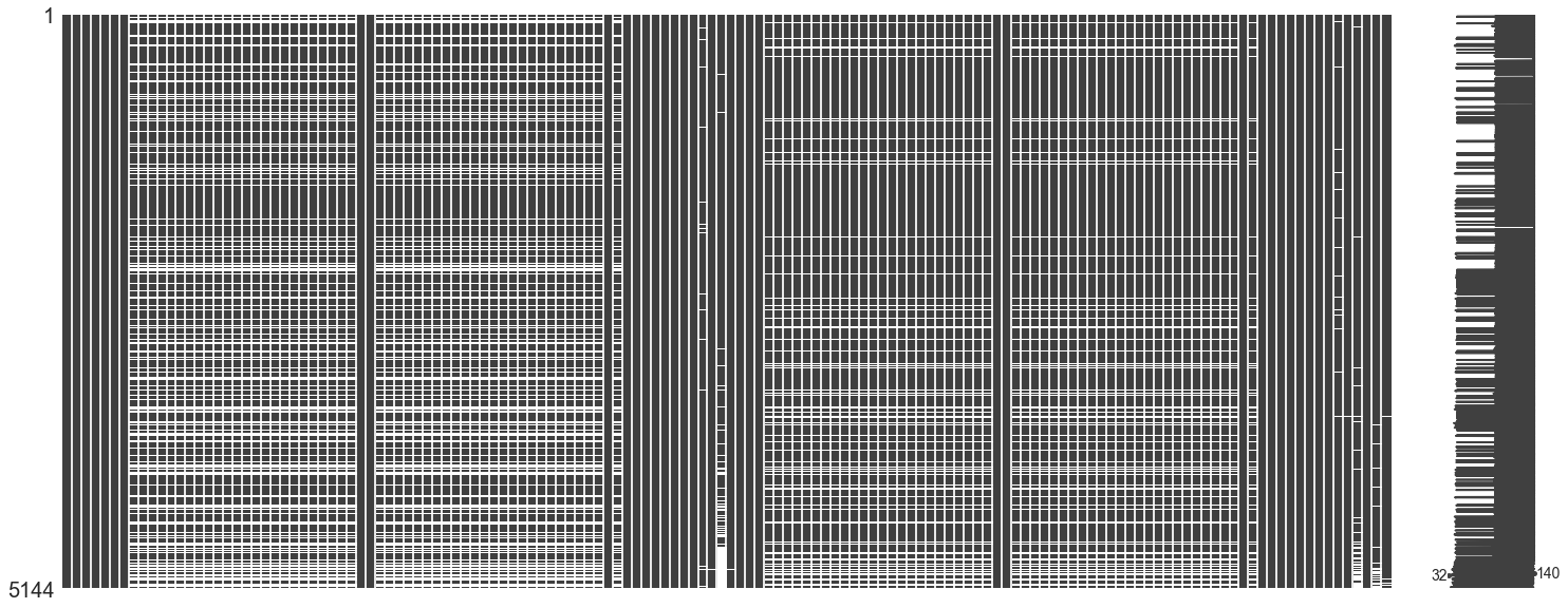
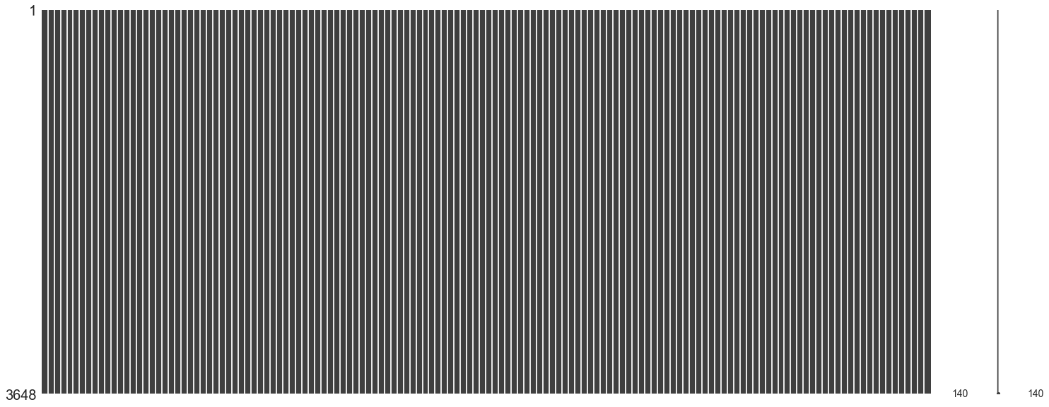
After looking at the website and .csv file directly, the missing values for AVGS appear to be for first fights in the UFC, as there is a '0' streak in the W/L columns for the appropriate row
## Visualizing the nulls, looking for patterns
mg.matrix(df);This confirms my initial thoughts visually, I will check one last time by filtering those without W/L streaks. (It may be useful later to make a column for first fighters)
Instead of making a new columns, for those without AVGs, I will fill them with 0's, to represent their 'UFC-only' stats. This could lead to issues later due to these fighters needing to have previous experience in MMA or combat sports in general. In order to net a spot on the fight card, it is likely there is data for them, but depending on numerous factors, in order to collect accurate data I would need to spend the time going through each individuals history.
Replacing Null Values:
- B/R_avg... & total_time = 0
- B/R_Stance = random choice acc. to probability
- B/R_Reach = groupby Height and use mean
- B/R_Height = groupby Reach and use mean
- B/R_Weight = groupby weight class and use mean
- B/R_age = mean
## Making list of cols to fill with 0 averages, then doing so
zero_fill_cols = [col for col in df.columns if 'avg' in col]
df_fill = df.copy()
df_fill[zero_fill_cols] = df_fill[zero_fill_cols].fillna(0)## Sanity check for filled nulls + visual
#pd.set_option('max_rows',None)
#print(df_fill.isna().sum())
mg.matrix(df_fill);## Checking distributions pt.1
df_fill['B_Stance'].value_counts(normalize=True)Orthodox 0.768104
Southpaw 0.195587
Switch 0.033701
Open Stance 0.001805
Sideways 0.000802
Name: B_Stance, dtype: float64
## Checking distributions pt.2
df_fill['R_Stance'].value_counts(normalize=True)Orthodox 0.759880
Southpaw 0.206786
Switch 0.029940
Open Stance 0.002994
Sideways 0.000399
Name: R_Stance, dtype: float64
## Making list for random choices
stance_list = list(df_fill['B_Stance'].dropna().unique())
print(stance_list)
## Making array of probabilities for corresp. stances
stance_ps = df_fill['R_Stance'].value_counts(normalize=True).values
print(stance_ps)['Orthodox', 'Switch', 'Southpaw', 'Open Stance', 'Sideways']
[7.59880240e-01 2.06786427e-01 2.99401198e-02 2.99401198e-03
3.99201597e-04]
## Using for loop to randomly fill stances according to probabilities
helper = ['B_Stance', 'R_Stance']
for col in helper:
df_fill[col] = df_fill[col].fillna(np.random.choice(stance_list, p=stance_ps))## Sanity check again
#pd.set_option('max_rows',None)
#print(df_fill.isna().sum())
mg.matrix(df_fill);Its getting better bit by bit!
## Using .groupby to find aggregrate stats for groups
height_grouped = df_fill.groupby('R_Height_cms').agg('mean')
display(height_grouped.head())
## Making dictionary of reach values acc. to height grouping
reach_by_height = dict(height_grouped['R_Reach_cms'])
display(reach_by_height).dataframe tbody tr th {
vertical-align: top;
}
.dataframe thead th {
text-align: right;
}
| title_bout | no_of_rounds | B_current_lose_streak | B_current_win_streak | B_draw | B_avg_BODY_att | B_avg_BODY_landed | B_avg_CLINCH_att | B_avg_CLINCH_landed | B_avg_DISTANCE_att | ... | R_win_by_Decision_Split | R_win_by_Decision_Unanimous | R_win_by_KO/TKO | R_win_by_Submission | R_win_by_TKO_Doctor_Stoppage | R_wins | R_Reach_cms | R_Weight_lbs | B_age | R_age | |
|---|---|---|---|---|---|---|---|---|---|---|---|---|---|---|---|---|---|---|---|---|---|
| R_Height_cms | |||||||||||||||||||||
| 152.40 | 0.000000 | 3.000000 | 0.000000 | 0.500000 | 0.0 | 8.750000 | 6.250000 | 8.500000 | 6.500000 | 71.750000 | ... | 1.000000 | 1.000000 | 0.000000 | 0.000000 | 0.000000 | 2.000000 | 152.400000 | 115.000000 | 26.500000 | 28.000000 |
| 154.94 | 0.080000 | 3.160000 | 0.280000 | 0.880000 | 0.0 | 12.076762 | 8.322000 | 14.464000 | 10.693238 | 64.446762 | ... | 0.400000 | 1.760000 | 0.160000 | 0.680000 | 0.000000 | 3.000000 | 157.480000 | 115.000000 | 29.160000 | 26.320000 |
| 157.48 | 0.000000 | 3.000000 | 0.714286 | 0.142857 | 0.0 | 3.214286 | 2.023810 | 3.190476 | 1.904762 | 53.333333 | ... | 0.000000 | 0.428571 | 0.000000 | 0.285714 | 0.000000 | 0.714286 | 160.745714 | 117.857143 | 29.714286 | 28.285714 |
| 160.02 | 0.190476 | 3.428571 | 0.349206 | 1.111111 | 0.0 | 12.551494 | 7.979525 | 8.324463 | 5.644547 | 64.666361 | ... | 0.507937 | 2.301587 | 1.238095 | 0.587302 | 0.095238 | 4.730159 | 164.858095 | 125.317460 | 28.349206 | 29.746032 |
| 162.56 | 0.035088 | 3.105263 | 0.324561 | 0.754386 | 0.0 | 9.453106 | 6.392813 | 8.522069 | 5.935818 | 56.728987 | ... | 0.219298 | 1.666667 | 0.473684 | 0.394737 | 0.000000 | 2.754386 | 164.987611 | 124.561404 | 28.552632 | 29.245614 |
5 rows × 135 columns
{152.4: 152.4,
154.94: 157.48000000000002,
157.48000000000005: 160.74571428571429,
160.02: 164.85809523809536,
162.56: 164.98761061946905,
165.1: 167.62145985401455,
167.64: 170.91507163323794,
170.18: 175.6790572390578,
172.72: 177.22211640211643,
175.26: 179.98928870292895,
177.8: 182.0478372591003,
180.34: 185.68854625550645,
182.88: 187.4072538860109,
185.42: 189.98413080895023,
187.96: 192.71544444444447,
190.5: 196.16033112582835,
193.04: 201.5994520547946,
195.58: 199.31062499999993,
198.12: 200.83517241379303,
200.66: 205.74,
203.2: 203.20000000000002,
208.28: nan,
210.82: 213.3600000000001}
## Same as above but targeting Height values to be filled
reach_grouped = df_fill.groupby('R_Reach_cms').agg('mean')
#display(reach_grouped)
height_by_reach = dict(reach_grouped['R_Height_cms'])
display(height_by_reach){152.4: 154.3755555555556,
157.48: 157.3106666666667,
160.02: 160.91370370370385,
162.56: 163.75944444444448,
165.1: 165.78914728682167,
167.64: 166.22531645569606,
170.18: 167.6562820512819,
172.72: 170.93834532374112,
175.26: 172.94302439024398,
177.8: 174.06380761523002,
180.34: 175.9309433962269,
182.88: 179.5954137115838,
185.42: 180.57549668874137,
187.96: 183.25398773006103,
190.5: 184.52804651162717,
193.04: 185.64592991913685,
195.58: 188.2499999999996,
198.12: 189.06991596638656,
200.66: 190.8122950819671,
203.2: 192.7577777777779,
205.74: 193.73272727272723,
208.28: 194.30999999999997,
210.82: 193.04,
213.36: 201.29499999999996}
## Targeting weight values to be filled
weight_cls_grouped = df_fill.groupby('weight_class').agg('mean')
#display(weight_cls_grouped)
weight_by_class = dict(weight_cls_grouped['R_Weight_lbs'])
display(weight_by_class){'Bantamweight': 134.5778364116095,
'Catch Weight': 183.5,
'Featherweight': 145.80316742081448,
'Flyweight': 127.13903743315508,
'Heavyweight': 245.10453648915188,
'Light Heavyweight': 202.5309381237525,
'Lightweight': 155.99291497975707,
'Middleweight': 184.72137931034482,
'Open Weight': 224.5164835164835,
'Welterweight': 170.312693498452,
"Women's Bantamweight": 133.64864864864865,
"Women's Featherweight": 145.0,
"Women's Flyweight": 125.0,
"Women's Strawweight": 116.53846153846153}
At this point I have the corresponding values for average height and reach based upon each other respectively in addition to average weight by weight class in dictionaries. Next I will use the .map() method to apply them appropriately.
## Scaffolding for filling of values
#df.B = df.B.fillna(df.A.map(dict))cols1 = ['B_Reach_cms', 'R_Reach_cms']
for col in cols1:
df_fill[col] = df_fill[col].fillna(df_fill['R_Height_cms'].map(reach_by_height))cols2 = ['B_Height_cms', 'R_Height_cms']
for col in cols2:
df_fill[col] = df_fill[col].fillna(df_fill['R_Reach_cms'].map(height_by_reach))cols3 = ['B_Weight_lbs', 'R_Weight_lbs']
for col in cols3:
df_fill[col] = df_fill[col].fillna(df_fill['weight_class'].map(weight_by_class))mg.matrix(df_fill);Needing to fill values that did not have Height nor Reach to fill from dictionary
## Locate the NAs Red corner
df_fill.loc[(pd.isnull(df_fill.R_Height_cms)), 'R_Height_cms']103 NaN
3607 NaN
5029 NaN
5132 NaN
Name: R_Height_cms, dtype: float64
## Verifying both columns are NA
list2 = [103, 3607, 5029, 5132]
for idx in list2:
display(df_fill.iloc[idx][['R_Height_cms', 'R_Reach_cms']])R_Height_cms NaN
R_Reach_cms NaN
Name: 103, dtype: object
R_Height_cms NaN
R_Reach_cms NaN
Name: 3607, dtype: object
R_Height_cms NaN
R_Reach_cms NaN
Name: 5029, dtype: object
R_Height_cms NaN
R_Reach_cms NaN
Name: 5132, dtype: object
## Locate the NAs Blue corner
df_fill.loc[(pd.isnull(df_fill.B_Height_cms)), 'B_Height_cms']4978 NaN
5020 NaN
5029 NaN
5134 NaN
Name: B_Height_cms, dtype: float64
## Same as above
list3 = [4978, 5020, 5029, 5134]
for idx in list3:
display(df_fill.iloc[idx][['B_Height_cms', 'B_Reach_cms']])B_Height_cms NaN
B_Reach_cms 185.689
Name: 4978, dtype: object
B_Height_cms NaN
B_Reach_cms 179.989
Name: 5020, dtype: object
B_Height_cms NaN
B_Reach_cms NaN
Name: 5029, dtype: object
B_Height_cms NaN
B_Reach_cms 192.715
Name: 5134, dtype: object
## Sanity check on specific index/help to make strategy to fill others
print(df_fill.iloc[3607].isna().sum())
df_fill.iloc[3607][['weight_class', 'R_Reach_cms', 'R_Height_cms', 'B_Reach_cms', 'B_Height_cms']]4
weight_class Light Heavyweight
R_Reach_cms NaN
R_Height_cms NaN
B_Reach_cms 190.5
B_Height_cms 190.5
Name: 3607, dtype: object
## Displaying values to fill according to each fight's weight class
## I have no other body attribute to go off of.
display(weight_cls_grouped[['R_Reach_cms', 'R_Height_cms', 'B_Reach_cms', 'B_Height_cms']].iloc[8])
display(weight_cls_grouped[['R_Reach_cms', 'R_Height_cms', 'B_Reach_cms', 'B_Height_cms']].iloc[6])
display(weight_cls_grouped[['R_Reach_cms', 'R_Height_cms', 'B_Reach_cms', 'B_Height_cms']].iloc[5])
display(weight_cls_grouped[['R_Reach_cms', 'R_Height_cms', 'B_Reach_cms', 'B_Height_cms']].iloc[4])R_Reach_cms 186.690000
R_Height_cms 186.424835
B_Reach_cms 182.880000
B_Height_cms 184.912000
Name: Open Weight, dtype: float64
R_Reach_cms 181.063807
R_Height_cms 176.481154
B_Reach_cms 181.392244
B_Height_cms 176.603492
Name: Lightweight, dtype: float64
R_Reach_cms 192.831803
R_Height_cms 187.137040
B_Reach_cms 192.145874
B_Height_cms 186.674821
Name: Light Heavyweight, dtype: float64
R_Reach_cms 196.393271
R_Height_cms 189.773570
B_Reach_cms 196.227178
B_Height_cms 189.827352
Name: Heavyweight, dtype: float64
Values to fill:
- Row 103 : Light Heavy R_Reach/Height ..... 2
- Row 3607: Light Heavy R_Reach/Height .... 2
- Row 4978: Lightweight B_Height ................ 1
- Row 5020: Heavyweight B_Height .............. 1
- Row 5029: Lightweight B/R_Reach/Height .. 4
- Row 5132: Open Weight B/R_Reach:R_Height . 3
- Row 5134: Open Weight B_Height ........... 1
## Creating dictionaries according to indices to fill the NAs from values above
val_R_rch = {103: 192.831803, 3607: 192.831803, 5029: 181.063807, 5132: 186.690000}
val_R_hgt = {103: 187.137040, 3607: 187.137040, 5029: 176.481154, 5132: 186.424835}
val_B_rch = {5029: 181.392244, 5132: 182.880000}
val_B_hgt = {4978: 176.603492, 5020: 189.827352, 5029: 176.603492, 5134: 184.912000}
## Filling each column acc. to dictionaries above
cols4 = ['R_Reach_cms', 'R_Height_cms', 'B_Reach_cms', 'B_Height_cms']
df_fill[cols4[0]] = df_fill[cols4[0]].fillna(val_R_rch)
df_fill[cols4[1]] = df_fill[cols4[1]].fillna(val_R_hgt)
df_fill[cols4[2]] = df_fill[cols4[2]].fillna(val_B_rch)
df_fill[cols4[3]] = df_fill[cols4[3]].fillna(val_B_hgt)mg.matrix(df_fill);#pd.set_option('max_rows', None)df_fill.isna().sum()Winner 0
title_bout 0
weight_class 0
no_of_rounds 0
B_current_lose_streak 0
B_current_win_streak 0
B_draw 0
B_avg_BODY_att 0
B_avg_BODY_landed 0
B_avg_CLINCH_att 0
B_avg_CLINCH_landed 0
B_avg_DISTANCE_att 0
B_avg_DISTANCE_landed 0
B_avg_GROUND_att 0
B_avg_GROUND_landed 0
B_avg_HEAD_att 0
B_avg_HEAD_landed 0
B_avg_KD 0
B_avg_LEG_att 0
B_avg_LEG_landed 0
B_avg_PASS 0
B_avg_REV 0
B_avg_SIG_STR_att 0
B_avg_SIG_STR_landed 0
B_avg_SIG_STR_pct 0
B_avg_SUB_ATT 0
B_avg_TD_att 0
B_avg_TD_landed 0
B_avg_TD_pct 0
B_avg_TOTAL_STR_att 0
...
R_avg_opp_KD 0
R_avg_opp_LEG_att 0
R_avg_opp_LEG_landed 0
R_avg_opp_PASS 0
R_avg_opp_REV 0
R_avg_opp_SIG_STR_att 0
R_avg_opp_SIG_STR_landed 0
R_avg_opp_SIG_STR_pct 0
R_avg_opp_SUB_ATT 0
R_avg_opp_TD_att 0
R_avg_opp_TD_landed 0
R_avg_opp_TD_pct 0
R_avg_opp_TOTAL_STR_att 0
R_avg_opp_TOTAL_STR_landed 0
R_total_rounds_fought 0
R_total_time_fought(seconds) 650
R_total_title_bouts 0
R_win_by_Decision_Majority 0
R_win_by_Decision_Split 0
R_win_by_Decision_Unanimous 0
R_win_by_KO/TKO 0
R_win_by_Submission 0
R_win_by_TKO_Doctor_Stoppage 0
R_wins 0
R_Stance 0
R_Height_cms 0
R_Reach_cms 3
R_Weight_lbs 0
B_age 172
R_age 64
Length: 140, dtype: int64
Almost there!
## Finding the rest
display(df_fill.loc[(pd.isnull(df_fill.R_Reach_cms)), 'R_Reach_cms'])
display(df_fill.loc[(pd.isnull(df_fill.B_Reach_cms)), 'B_Reach_cms'])4800 NaN
4814 NaN
4883 NaN
Name: R_Reach_cms, dtype: float64
4800 NaN
4814 NaN
4883 NaN
Name: B_Reach_cms, dtype: float64
I am going to find the weight classes and confirm the values I need to fill.
print(df_fill.iloc[4800].isna().sum())
df_fill.iloc[4800][['weight_class', 'R_Reach_cms', 'B_Reach_cms']]2
weight_class Heavyweight
R_Reach_cms NaN
B_Reach_cms NaN
Name: 4800, dtype: object
print(df_fill.iloc[4814].isna().sum())
df_fill.iloc[4814][['weight_class', 'R_Reach_cms', 'B_Reach_cms']]2
weight_class Heavyweight
R_Reach_cms NaN
B_Reach_cms NaN
Name: 4814, dtype: object
print(df_fill.iloc[4883].isna().sum())
df_fill.iloc[4883][['weight_class', 'R_Reach_cms', 'B_Reach_cms']]3
weight_class Heavyweight
R_Reach_cms NaN
B_Reach_cms NaN
Name: 4883, dtype: object
## Grabbing avgs. from groupby to fill with
display(weight_cls_grouped[['R_Reach_cms', 'B_Reach_cms']].iloc[4])R_Reach_cms 196.393271
B_Reach_cms 196.227178
Name: Heavyweight, dtype: float64
## Same as above
val_R_rch2 = {4800: 196.393271, 4814: 196.393271, 4883: 196.393271}
val_B_rch2 = {4800: 196.227178, 4814: 196.227178, 4883: 196.227178}
## For reference
#cols4 = ['R_Reach_cms', 'R_Height_cms', 'B_Reach_cms', 'B_Height_cms']
df_fill[cols4[0]] = df_fill[cols4[0]].fillna(val_R_rch2)
df_fill[cols4[2]] = df_fill[cols4[2]].fillna(val_B_rch2)#pd.set_option('max_rows', None)df_fill.isna().sum()Winner 0
title_bout 0
weight_class 0
no_of_rounds 0
B_current_lose_streak 0
B_current_win_streak 0
B_draw 0
B_avg_BODY_att 0
B_avg_BODY_landed 0
B_avg_CLINCH_att 0
B_avg_CLINCH_landed 0
B_avg_DISTANCE_att 0
B_avg_DISTANCE_landed 0
B_avg_GROUND_att 0
B_avg_GROUND_landed 0
B_avg_HEAD_att 0
B_avg_HEAD_landed 0
B_avg_KD 0
B_avg_LEG_att 0
B_avg_LEG_landed 0
B_avg_PASS 0
B_avg_REV 0
B_avg_SIG_STR_att 0
B_avg_SIG_STR_landed 0
B_avg_SIG_STR_pct 0
B_avg_SUB_ATT 0
B_avg_TD_att 0
B_avg_TD_landed 0
B_avg_TD_pct 0
B_avg_TOTAL_STR_att 0
...
R_avg_opp_KD 0
R_avg_opp_LEG_att 0
R_avg_opp_LEG_landed 0
R_avg_opp_PASS 0
R_avg_opp_REV 0
R_avg_opp_SIG_STR_att 0
R_avg_opp_SIG_STR_landed 0
R_avg_opp_SIG_STR_pct 0
R_avg_opp_SUB_ATT 0
R_avg_opp_TD_att 0
R_avg_opp_TD_landed 0
R_avg_opp_TD_pct 0
R_avg_opp_TOTAL_STR_att 0
R_avg_opp_TOTAL_STR_landed 0
R_total_rounds_fought 0
R_total_time_fought(seconds) 650
R_total_title_bouts 0
R_win_by_Decision_Majority 0
R_win_by_Decision_Split 0
R_win_by_Decision_Unanimous 0
R_win_by_KO/TKO 0
R_win_by_Submission 0
R_win_by_TKO_Doctor_Stoppage 0
R_wins 0
R_Stance 0
R_Height_cms 0
R_Reach_cms 0
R_Weight_lbs 0
B_age 172
R_age 64
Length: 140, dtype: int64
mg.matrix(df_fill);## Creating variable to hold age mean for filling
print(df_fill[['B_age', 'R_age']].mean())
## Taking midpoint between two columns
age_mean = (df_fill['B_age'].mean() + df_fill['R_age'].mean()) / 2
age_meanB_age 29.171963
R_age 29.442323
dtype: float64
29.307142913702563
## Filling with mean age
df_fill['B_age'] = df_fill['B_age'].fillna(age_mean)
df_fill['R_age'] = df_fill['R_age'].fillna(age_mean)Filled age with mean, looking at those rows, generally speaking, it appears that first time fighters are the culprit again. This may have to do with the lack of preplanning or rescheduling due to injury.
## Visual check
mg.matrix(df_fill);## Filling with zeros for first time fighters
df_fill['R_total_time_fought(seconds)'] = df_fill['R_total_time_fought(seconds)'].fillna(0)
df_fill['B_total_time_fought(seconds)'] = df_fill['B_total_time_fought(seconds)'].fillna(0)## Null check
#print(df_fill.isna().sum())
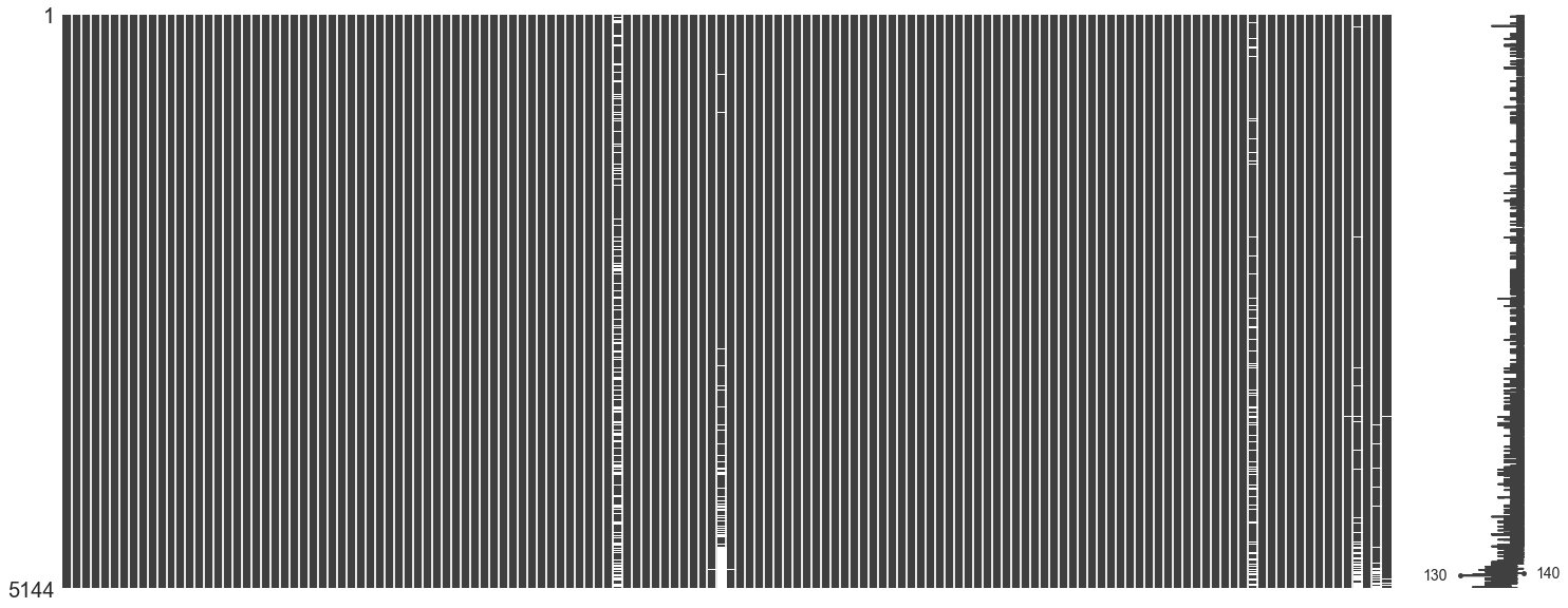
mg.matrix(df_fill);Finally done!
## Check for categories and peek at Df
print(df_fill.info())
df_fill.select_dtypes(['object', 'bool']).head()<class 'pandas.core.frame.DataFrame'>
RangeIndex: 5144 entries, 0 to 5143
Columns: 140 entries, Winner to R_age
dtypes: bool(1), float64(134), int64(1), object(4)
memory usage: 5.5+ MB
None
.dataframe tbody tr th {
    vertical-align: top;
}

.dataframe thead th {
    text-align: right;
}
| Winner | title_bout | weight_class | B_Stance | R_Stance | |
|---|---|---|---|---|---|
| 0 | Red | True | Bantamweight | Orthodox | Orthodox |
| 1 | Red | True | Women's Flyweight | Orthodox | Southpaw |
| 2 | Red | False | Lightweight | Orthodox | Orthodox |
| 3 | Blue | False | Bantamweight | Switch | Orthodox |
| 4 | Blue | False | Heavyweight | Southpaw | Southpaw |
## Encoding categorical columns
cat_df = df_fill.select_dtypes(['object', 'bool']).copy()
dummy_df = pd.get_dummies(cat_df)
## Dropping title to reintroduce as an int and Winner as label encoded
dummy_df.drop(columns=['title_bout', 'Winner_Blue', 'Winner_Draw', 'Winner_Red'], inplace=True)
dummy_df.head().dataframe tbody tr th {
vertical-align: top;
}
.dataframe thead th {
text-align: right;
}
| weight_class_Bantamweight | weight_class_Catch Weight | weight_class_Featherweight | weight_class_Flyweight | weight_class_Heavyweight | weight_class_Light Heavyweight | weight_class_Lightweight | weight_class_Middleweight | weight_class_Open Weight | weight_class_Welterweight | ... | B_Stance_Open Stance | B_Stance_Orthodox | B_Stance_Sideways | B_Stance_Southpaw | B_Stance_Switch | R_Stance_Open Stance | R_Stance_Orthodox | R_Stance_Sideways | R_Stance_Southpaw | R_Stance_Switch | |
|---|---|---|---|---|---|---|---|---|---|---|---|---|---|---|---|---|---|---|---|---|---|
| 0 | 1 | 0 | 0 | 0 | 0 | 0 | 0 | 0 | 0 | 0 | ... | 0 | 1 | 0 | 0 | 0 | 0 | 1 | 0 | 0 | 0 |
| 1 | 0 | 0 | 0 | 0 | 0 | 0 | 0 | 0 | 0 | 0 | ... | 0 | 1 | 0 | 0 | 0 | 0 | 0 | 0 | 1 | 0 |
| 2 | 0 | 0 | 0 | 0 | 0 | 0 | 1 | 0 | 0 | 0 | ... | 0 | 1 | 0 | 0 | 0 | 0 | 1 | 0 | 0 | 0 |
| 3 | 1 | 0 | 0 | 0 | 0 | 0 | 0 | 0 | 0 | 0 | ... | 0 | 0 | 0 | 0 | 1 | 0 | 1 | 0 | 0 | 0 |
| 4 | 0 | 0 | 0 | 0 | 1 | 0 | 0 | 0 | 0 | 0 | ... | 0 | 0 | 0 | 1 | 0 | 0 | 0 | 0 | 1 | 0 |
5 rows × 24 columns
## Series to label encoding winner column
win_series = cat_df['Winner'].copy()
dict_win = {'Draw': 0, 'Red': 1, 'Blue': 2}
win_series = win_series.map(dict_win)
win_series.value_counts()1 3470
2 1591
0 83
Name: Winner, dtype: int64
## Same as winner column
title_series = cat_df['title_bout'].copy()
dict_title = {True: 1, False: 0}
title_series = title_series.map(dict_title)
title_series.head()0 1
1 1
2 0
3 0
4 0
Name: title_bout, dtype: int64
## Helper for code length
drop_cols = ['Winner', 'title_bout', 'B_Stance', 'R_Stance', 'weight_class']## Putting it back together
df_full = pd.concat([df_fill.drop(columns=drop_cols), win_series, title_series, dummy_df], axis=1)
df_full.head().dataframe tbody tr th {
vertical-align: top;
}
.dataframe thead th {
text-align: right;
}
| no_of_rounds | B_current_lose_streak | B_current_win_streak | B_draw | B_avg_BODY_att | B_avg_BODY_landed | B_avg_CLINCH_att | B_avg_CLINCH_landed | B_avg_DISTANCE_att | B_avg_DISTANCE_landed | ... | B_Stance_Open Stance | B_Stance_Orthodox | B_Stance_Sideways | B_Stance_Southpaw | B_Stance_Switch | R_Stance_Open Stance | R_Stance_Orthodox | R_Stance_Sideways | R_Stance_Southpaw | R_Stance_Switch | |
|---|---|---|---|---|---|---|---|---|---|---|---|---|---|---|---|---|---|---|---|---|---|
| 0 | 5 | 0.0 | 4.0 | 0.0 | 9.200000 | 6.000000 | 0.200000 | 0.000000 | 62.600000 | 20.600000 | ... | 0 | 1 | 0 | 0 | 0 | 0 | 1 | 0 | 0 | 0 |
| 1 | 5 | 0.0 | 3.0 | 0.0 | 14.600000 | 9.100000 | 11.800000 | 7.300000 | 124.700000 | 42.100000 | ... | 0 | 1 | 0 | 0 | 0 | 0 | 0 | 0 | 1 | 0 |
| 2 | 3 | 0.0 | 3.0 | 0.0 | 15.354839 | 11.322581 | 6.741935 | 4.387097 | 84.741935 | 38.580645 | ... | 0 | 1 | 0 | 0 | 0 | 0 | 1 | 0 | 0 | 0 |
| 3 | 3 | 0.0 | 4.0 | 0.0 | 17.000000 | 14.000000 | 13.750000 | 11.000000 | 109.500000 | 48.750000 | ... | 0 | 0 | 0 | 0 | 1 | 0 | 1 | 0 | 0 | 0 |
| 4 | 3 | 0.0 | 1.0 | 0.0 | 17.000000 | 14.500000 | 2.500000 | 2.000000 | 201.000000 | 59.500000 | ... | 0 | 0 | 0 | 1 | 0 | 0 | 0 | 0 | 1 | 0 |
5 rows × 161 columns
df_full.info()<class 'pandas.core.frame.DataFrame'>
RangeIndex: 5144 entries, 0 to 5143
Columns: 161 entries, no_of_rounds to R_Stance_Switch
dtypes: float64(134), int64(3), uint8(24)
memory usage: 5.5 MB
## Set up for quick visual check of multicollinearity
corr_test = df_full.corr()fig, ax = plt.subplots(figsize=(12,12))
sns.heatmap(corr_test, vmin=-1, vmax=1, center=0,
cmap=sns.diverging_palette(20, 220, n=200), square=True)
ax.set_xticklabels(ax.get_xticklabels(), rotation=45,
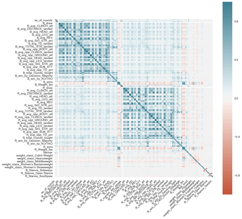
horizontalalignment='right');AVGS show some correlation, but nothing demonstrates a strong connection to the winner category
In order to explore different types of models, it is imperative to scale data to allow for proper calculations.
## Separate features from target to train-test split
X = df_full.drop('Winner', axis=1).copy()
y = df_full['Winner'].copy()
X_train, X_test, y_train, y_test = train_test_split(X, y, random_state=22)I performed the split prior to scaling to prevent leakage into my test data set
## Verifying class balance is roughly the same
print('Original Class Balance')
display(y.value_counts(normalize=True))
print('y_train Class Balance')
display(y_train.value_counts(normalize=True))
print('y_test Class Balance')
display(y_test.value_counts(normalize=True))Original Class Balance
1 0.674572
2 0.309292
0 0.016135
Name: Winner, dtype: float64
y_train Class Balance
1 0.680404
2 0.304044
0 0.015552
Name: Winner, dtype: float64
y_test Class Balance
1 0.657076
2 0.325039
0 0.017885
Name: Winner, dtype: float64
## Instantiate scaler and fit_transform to training only
scaler = MinMaxScaler()
X_train_sca = pd.DataFrame(scaler.fit_transform(X_train), columns=X_train.columns,
index=X_train.index)
X_test_sca = pd.DataFrame(scaler.transform(X_test), columns=X_test.columns,
index=X_test.index)
## Check for scaling
display(X_train_sca.head())
display(X_train_sca.describe().loc[['min', 'max']])
display(X_test_sca.head())
display(X_test_sca.describe().loc[['min', 'max']]).dataframe tbody tr th {
vertical-align: top;
}
.dataframe thead th {
text-align: right;
}
| no_of_rounds | B_current_lose_streak | B_current_win_streak | B_draw | B_avg_BODY_att | B_avg_BODY_landed | B_avg_CLINCH_att | B_avg_CLINCH_landed | B_avg_DISTANCE_att | B_avg_DISTANCE_landed | ... | B_Stance_Open Stance | B_Stance_Orthodox | B_Stance_Sideways | B_Stance_Southpaw | B_Stance_Switch | R_Stance_Open Stance | R_Stance_Orthodox | R_Stance_Sideways | R_Stance_Southpaw | R_Stance_Switch | |
|---|---|---|---|---|---|---|---|---|---|---|---|---|---|---|---|---|---|---|---|---|---|
| 2898 | 1.0 | 0.0 | 0.076923 | 0.0 | 0.167347 | 0.164103 | 0.062069 | 0.050000 | 0.325461 | 0.262009 | ... | 0.0 | 1.0 | 0.0 | 0.0 | 0.0 | 0.0 | 1.0 | 0.0 | 0.0 | 0.0 |
| 1358 | 0.5 | 0.0 | 0.000000 | 0.0 | 0.000000 | 0.000000 | 0.000000 | 0.000000 | 0.000000 | 0.000000 | ... | 0.0 | 1.0 | 0.0 | 0.0 | 0.0 | 0.0 | 1.0 | 0.0 | 0.0 | 0.0 |
| 2510 | 0.5 | 0.0 | 0.230769 | 0.0 | 0.292517 | 0.247863 | 0.045977 | 0.039216 | 0.554736 | 0.509461 | ... | 0.0 | 1.0 | 0.0 | 0.0 | 0.0 | 0.0 | 1.0 | 0.0 | 0.0 | 0.0 |
| 1181 | 0.5 | 0.0 | 0.230769 | 0.0 | 0.119898 | 0.073718 | 0.043103 | 0.034926 | 0.193727 | 0.117904 | ... | 0.0 | 1.0 | 0.0 | 0.0 | 0.0 | 0.0 | 1.0 | 0.0 | 0.0 | 0.0 |
| 4583 | 0.5 | 0.0 | 0.000000 | 0.0 | 0.000000 | 0.000000 | 0.000000 | 0.000000 | 0.000000 | 0.000000 | ... | 0.0 | 1.0 | 0.0 | 0.0 | 0.0 | 0.0 | 1.0 | 0.0 | 0.0 | 0.0 |
5 rows × 160 columns
.dataframe tbody tr th {
    vertical-align: top;
}

.dataframe thead th {
    text-align: right;
}
| no_of_rounds | B_current_lose_streak | B_current_win_streak | B_draw | B_avg_BODY_att | B_avg_BODY_landed | B_avg_CLINCH_att | B_avg_CLINCH_landed | B_avg_DISTANCE_att | B_avg_DISTANCE_landed | ... | B_Stance_Open Stance | B_Stance_Orthodox | B_Stance_Sideways | B_Stance_Southpaw | B_Stance_Switch | R_Stance_Open Stance | R_Stance_Orthodox | R_Stance_Sideways | R_Stance_Southpaw | R_Stance_Switch | |
|---|---|---|---|---|---|---|---|---|---|---|---|---|---|---|---|---|---|---|---|---|---|
| min | 0.0 | 0.0 | 0.0 | 0.0 | 0.0 | 0.0 | 0.0 | 0.0 | 0.0 | 0.0 | ... | 0.0 | 0.0 | 0.0 | 0.0 | 0.0 | 0.0 | 0.0 | 0.0 | 0.0 | 0.0 |
| max | 1.0 | 1.0 | 1.0 | 0.0 | 1.0 | 1.0 | 1.0 | 1.0 | 1.0 | 1.0 | ... | 1.0 | 1.0 | 1.0 | 1.0 | 1.0 | 1.0 | 1.0 | 1.0 | 1.0 | 1.0 |
2 rows × 160 columns
.dataframe tbody tr th {
    vertical-align: top;
}

.dataframe thead th {
    text-align: right;
}
| no_of_rounds | B_current_lose_streak | B_current_win_streak | B_draw | B_avg_BODY_att | B_avg_BODY_landed | B_avg_CLINCH_att | B_avg_CLINCH_landed | B_avg_DISTANCE_att | B_avg_DISTANCE_landed | ... | B_Stance_Open Stance | B_Stance_Orthodox | B_Stance_Sideways | B_Stance_Southpaw | B_Stance_Switch | R_Stance_Open Stance | R_Stance_Orthodox | R_Stance_Sideways | R_Stance_Southpaw | R_Stance_Switch | |
|---|---|---|---|---|---|---|---|---|---|---|---|---|---|---|---|---|---|---|---|---|---|
| 1899 | 0.5 | 0.166667 | 0.000000 | 0.0 | 0.104308 | 0.095442 | 0.075990 | 0.070261 | 0.114801 | 0.116934 | ... | 0.0 | 1.0 | 0.0 | 0.0 | 0.0 | 0.0 | 0.0 | 0.0 | 1.0 | 0.0 |
| 4061 | 0.5 | 0.000000 | 0.000000 | 0.0 | 0.000000 | 0.000000 | 0.000000 | 0.000000 | 0.000000 | 0.000000 | ... | 0.0 | 1.0 | 0.0 | 0.0 | 0.0 | 0.0 | 1.0 | 0.0 | 0.0 | 0.0 |
| 1831 | 1.0 | 0.000000 | 0.384615 | 0.0 | 0.061224 | 0.043393 | 0.045977 | 0.032805 | 0.150724 | 0.104132 | ... | 0.0 | 1.0 | 0.0 | 0.0 | 0.0 | 0.0 | 1.0 | 0.0 | 0.0 | 0.0 |
| 1788 | 0.5 | 0.166667 | 0.000000 | 0.0 | 0.215743 | 0.179487 | 0.067323 | 0.046218 | 0.191355 | 0.193387 | ... | 0.0 | 1.0 | 0.0 | 0.0 | 0.0 | 0.0 | 1.0 | 0.0 | 0.0 | 0.0 |
| 5088 | 0.0 | 0.000000 | 0.000000 | 0.0 | 0.000000 | 0.000000 | 0.000000 | 0.000000 | 0.000000 | 0.000000 | ... | 0.0 | 1.0 | 0.0 | 0.0 | 0.0 | 0.0 | 1.0 | 0.0 | 0.0 | 0.0 |
5 rows × 160 columns
.dataframe tbody tr th {
    vertical-align: top;
}

.dataframe thead th {
    text-align: right;
}
| no_of_rounds | B_current_lose_streak | B_current_win_streak | B_draw | B_avg_BODY_att | B_avg_BODY_landed | B_avg_CLINCH_att | B_avg_CLINCH_landed | B_avg_DISTANCE_att | B_avg_DISTANCE_landed | ... | B_Stance_Open Stance | B_Stance_Orthodox | B_Stance_Sideways | B_Stance_Southpaw | B_Stance_Switch | R_Stance_Open Stance | R_Stance_Orthodox | R_Stance_Sideways | R_Stance_Southpaw | R_Stance_Switch | |
|---|---|---|---|---|---|---|---|---|---|---|---|---|---|---|---|---|---|---|---|---|---|
| min | 0.0 | 0.000000 | 0.000000 | 0.0 | 0.000000 | 0.000000 | 0.00000 | 0.000000 | 0.0 | 0.000000 | ... | 0.0 | 0.0 | 0.0 | 0.0 | 0.0 | 0.0 | 0.0 | 0.0 | 0.0 | 0.0 |
| max | 1.0 | 0.833333 | 0.615385 | 0.0 | 0.979592 | 0.717949 | 0.54023 | 0.544118 | 1.0 | 1.135371 | ... | 1.0 | 1.0 | 1.0 | 1.0 | 1.0 | 1.0 | 1.0 | 0.0 | 1.0 | 1.0 |
2 rows × 160 columns
## Instantiating a bunch of classifiers to test
tree_clf = DecisionTreeClassifier(class_weight='balanced')
rf_clf = RandomForestClassifier(class_weight='balanced')
log_clf = LogisticRegression(C=1e9, class_weight='balanced',
multi_class='multinomial')
knn_clf = KNeighborsClassifier()
ada_clf = AdaBoostClassifier()
grad_clf = GradientBoostingClassifier()
xgb_clf = xgb.XGBClassifier(objective='multi:softprob', num_class=3)## Set up to time models/check performance
mods = [log_clf, tree_clf, rf_clf, knn_clf, ada_clf, grad_clf, xgb_clf]
mod_labs = ['log_clf', 'tree_clf', 'rf_clf', 'knn_clf', 'ada_clf', 'grad_clf', 'xgb_clf']
t = dlf.Timer()
labs = ['draw', 'Red - Win', 'Blue - Win']
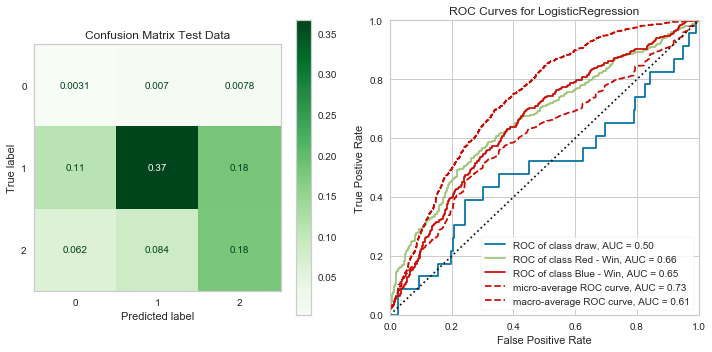
times = dlf.time_models(X_train_sca, X_test_sca, y_train, y_test, mods, mod_labs, t, cls_lab=labs)LogisticRegression(C=1000000000.0, class_weight='balanced', dual=False,
fit_intercept=True, intercept_scaling=1, l1_ratio=None,
max_iter=100, multi_class='multinomial', n_jobs=None,
penalty='l2', random_state=None, solver='lbfgs', tol=0.0001,
verbose=0, warm_start=False)
Classification Report Test
precision recall f1-score support
0 0.02 0.17 0.03 23
1 0.80 0.56 0.66 845
2 0.49 0.55 0.52 418
accuracy 0.55 1286
macro avg 0.44 0.43 0.40 1286
weighted avg 0.68 0.55 0.60 1286
---- Timer stopped at: 04/27/2020 - 08:43 PM ----
---- Time elasped: 0:00:01.132971 ----
DecisionTreeClassifier(ccp_alpha=0.0, class_weight='balanced', criterion='gini',
max_depth=None, max_features=None, max_leaf_nodes=None,
min_impurity_decrease=0.0, min_impurity_split=None,
min_samples_leaf=1, min_samples_split=2,
min_weight_fraction_leaf=0.0, presort='deprecated',
random_state=None, splitter='best')
Classification Report Test
precision recall f1-score support
0 0.00 0.00 0.00 23
1 0.68 0.70 0.69 845
2 0.38 0.36 0.37 418
accuracy 0.58 1286
macro avg 0.36 0.36 0.36 1286
weighted avg 0.57 0.58 0.58 1286
---- Timer stopped at: 04/27/2020 - 08:43 PM ----
---- Time elasped: 0:00:01.170899 ----
RandomForestClassifier(bootstrap=True, ccp_alpha=0.0, class_weight='balanced',
criterion='gini', max_depth=None, max_features='auto',
max_leaf_nodes=None, max_samples=None,
min_impurity_decrease=0.0, min_impurity_split=None,
min_samples_leaf=1, min_samples_split=2,
min_weight_fraction_leaf=0.0, n_estimators=100,
n_jobs=None, oob_score=False, random_state=None,
verbose=0, warm_start=False)
Classification Report Test
precision recall f1-score support
0 0.00 0.00 0.00 23
1 0.67 0.97 0.79 845
2 0.60 0.09 0.16 418
accuracy 0.67 1286
macro avg 0.42 0.35 0.32 1286
weighted avg 0.64 0.67 0.57 1286
---- Timer stopped at: 04/27/2020 - 08:43 PM ----
---- Time elasped: 0:00:03.938470 ----
KNeighborsClassifier(algorithm='auto', leaf_size=30, metric='minkowski',
metric_params=None, n_jobs=None, n_neighbors=5, p=2,
weights='uniform')
Classification Report Test
precision recall f1-score support
0 0.00 0.00 0.00 23
1 0.68 0.82 0.74 845
2 0.41 0.26 0.32 418
accuracy 0.62 1286
macro avg 0.36 0.36 0.35 1286
weighted avg 0.58 0.62 0.59 1286
---- Timer stopped at: 04/27/2020 - 08:43 PM ----
---- Time elasped: 0:00:19.038378 ----
AdaBoostClassifier(algorithm='SAMME.R', base_estimator=None, learning_rate=1.0,
n_estimators=50, random_state=None)
Classification Report Test
precision recall f1-score support
0 0.00 0.00 0.00 23
1 0.68 0.92 0.78 845
2 0.51 0.18 0.26 418
accuracy 0.66 1286
macro avg 0.40 0.36 0.35 1286
weighted avg 0.61 0.66 0.60 1286
---- Timer stopped at: 04/27/2020 - 08:43 PM ----
---- Time elasped: 0:00:02.523258 ----
GradientBoostingClassifier(ccp_alpha=0.0, criterion='friedman_mse', init=None,
learning_rate=0.1, loss='deviance', max_depth=3,
max_features=None, max_leaf_nodes=None,
min_impurity_decrease=0.0, min_impurity_split=None,
min_samples_leaf=1, min_samples_split=2,
min_weight_fraction_leaf=0.0, n_estimators=100,
n_iter_no_change=None, presort='deprecated',
random_state=None, subsample=1.0, tol=0.0001,
validation_fraction=0.1, verbose=0,
warm_start=False)
Classification Report Test
precision recall f1-score support
0 0.00 0.00 0.00 23
1 0.69 0.91 0.79 845
2 0.54 0.22 0.32 418
accuracy 0.67 1286
macro avg 0.41 0.38 0.37 1286
weighted avg 0.63 0.67 0.62 1286
---- Timer stopped at: 04/27/2020 - 08:44 PM ----
---- Time elasped: 0:00:26.651734 ----
XGBClassifier(base_score=0.5, booster='gbtree', colsample_bylevel=1,
colsample_bytree=1, gamma=0, learning_rate=0.1, max_delta_step=0,
max_depth=3, min_child_weight=1, missing=None, n_estimators=100,
n_jobs=1, nthread=None, num_class=3, objective='multi:softprob',
random_state=0, reg_alpha=0, reg_lambda=1, scale_pos_weight=1,
seed=None, silent=True, subsample=1)
Classification Report Test
precision recall f1-score support
0 0.00 0.00 0.00 23
1 0.69 0.92 0.79 845
2 0.55 0.21 0.31 418
accuracy 0.67 1286
macro avg 0.41 0.38 0.36 1286
weighted avg 0.63 0.67 0.62 1286
---- Timer stopped at: 04/27/2020 - 08:44 PM ----
---- Time elasped: 0:00:07.353348 ----
# Check for run-times
times_sorted = sorted(times.items(), key=lambda x: x[1])
times_sorted[('log_clf', 1.132971),
('tree_clf', 1.170899),
('ada_clf', 2.523258),
('rf_clf', 3.93847),
('xgb_clf', 7.353348),
('knn_clf', 19.038378),
('grad_clf', 26.651734)]
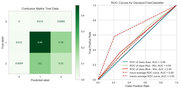
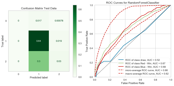
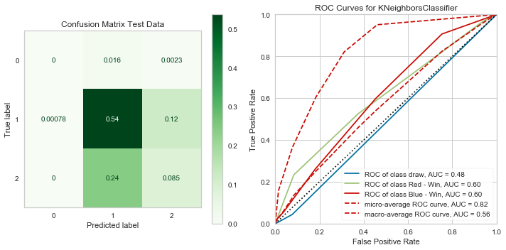
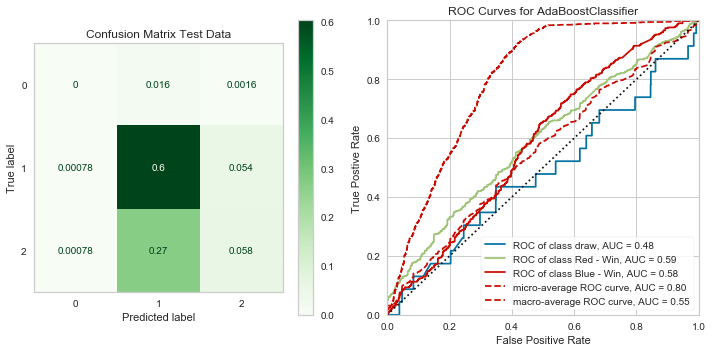
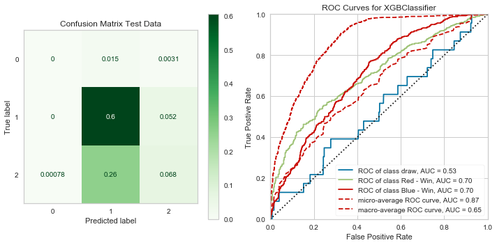
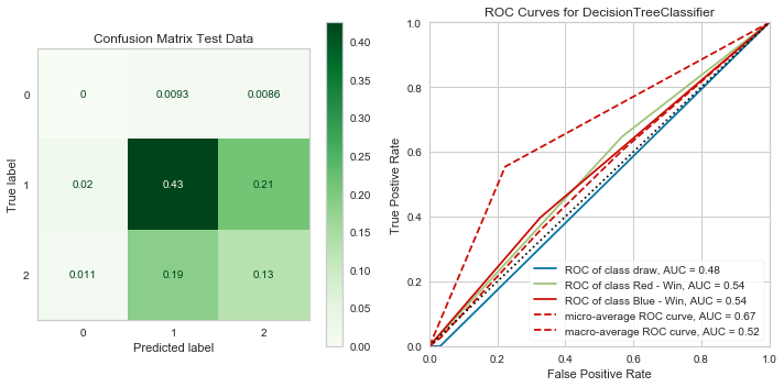
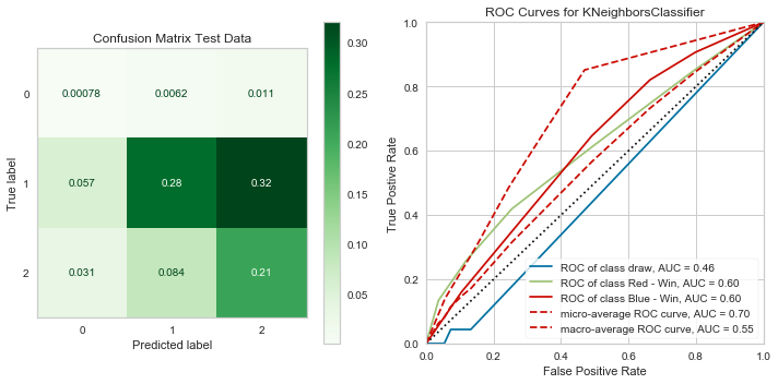
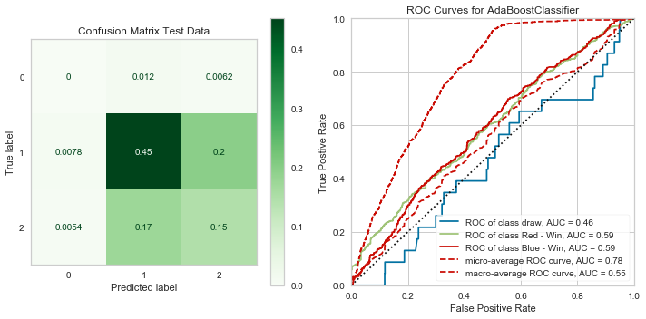
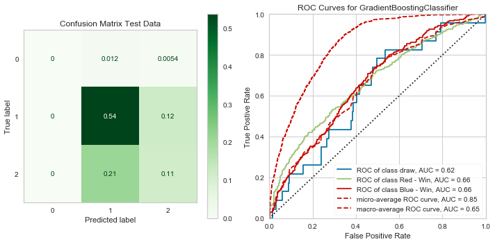
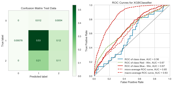
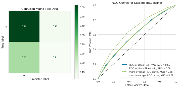
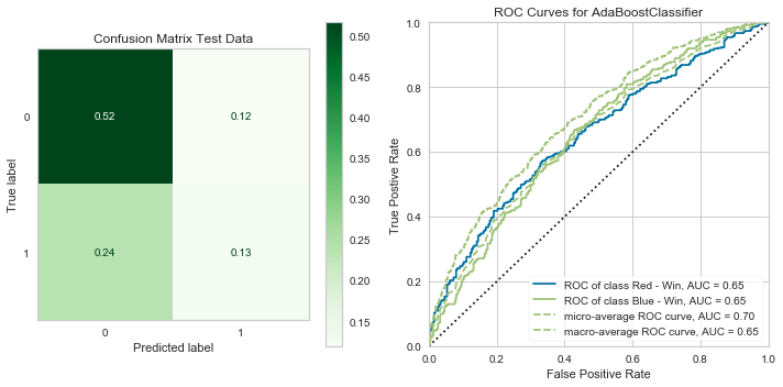
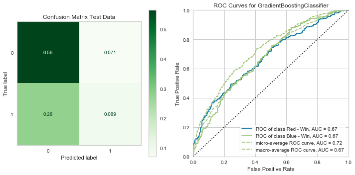
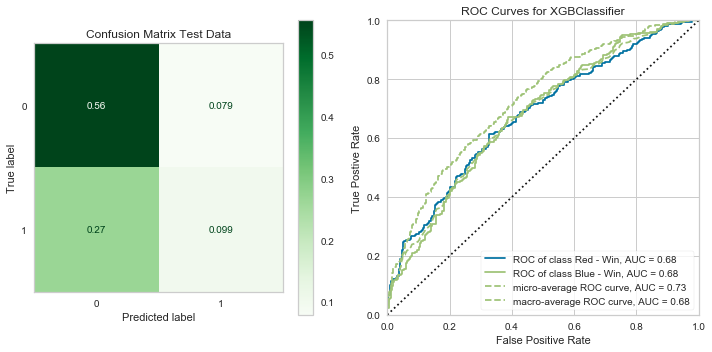
I have good accuracy, but it is misleading because it is almost always guessing class 1, which due to class imbalances is likely to be right when it does. Next I will try and remedy this.
My classifiers may be missing so much due to the class imbalances for the categories, I am going to oversample the minority classes in order to compensate.
print('Original class distribution: \n')
print(y_train.value_counts())
smote = SMOTE()
X_trn_sca_resmp, y_trn_resmp = smote.fit_sample(X_train_sca, y_train)
X_trn_sca_resmp = pd.DataFrame(X_trn_sca_resmp, columns=X_train_sca.columns)
print('-----------------------------------------')
print('Resampled class distribution: \n')
print(pd.Series(y_trn_resmp).value_counts()) Original class distribution:
1 2625
2 1173
0 60
Name: Winner, dtype: int64
-----------------------------------------
Resampled class distribution:
2 2625
1 2625
0 2625
dtype: int64
## Model check
mods = [log_clf, tree_clf, rf_clf, knn_clf, ada_clf, grad_clf, xgb_clf]
mod_labs = ['log_clf', 'tree_clf', 'rf_clf', 'knn_clf', 'ada_clf', 'grad_clf', 'xgb_clf']
t = dlf.Timer()
labs = ['draw', 'Red - Win', 'Blue - Win']
times = dlf.time_models(X_trn_sca_resmp, X_test_sca, y_trn_resmp, y_test, mods, mod_labs, t, cls_lab=labs)LogisticRegression(C=1000000000.0, class_weight='balanced', dual=False,
fit_intercept=True, intercept_scaling=1, l1_ratio=None,
max_iter=100, multi_class='multinomial', n_jobs=None,
penalty='l2', random_state=None, solver='lbfgs', tol=0.0001,
verbose=0, warm_start=False)
Classification Report Test
precision recall f1-score support
0 0.02 0.17 0.03 23
1 0.79 0.57 0.66 845
2 0.48 0.52 0.50 418
accuracy 0.55 1286
macro avg 0.43 0.42 0.40 1286
weighted avg 0.67 0.55 0.60 1286
---- Timer stopped at: 04/27/2020 - 08:46 PM ----
---- Time elasped: 0:00:01.187388 ----
DecisionTreeClassifier(ccp_alpha=0.0, class_weight='balanced', criterion='gini',
max_depth=None, max_features=None, max_leaf_nodes=None,
min_impurity_decrease=0.0, min_impurity_split=None,
min_samples_leaf=1, min_samples_split=2,
min_weight_fraction_leaf=0.0, presort='deprecated',
random_state=None, splitter='best')
Classification Report Test
precision recall f1-score support
0 0.00 0.00 0.00 23
1 0.69 0.65 0.67 845
2 0.37 0.40 0.38 418
accuracy 0.55 1286
macro avg 0.35 0.35 0.35 1286
weighted avg 0.57 0.55 0.56 1286
---- Timer stopped at: 04/27/2020 - 08:46 PM ----
---- Time elasped: 0:00:01.864052 ----
RandomForestClassifier(bootstrap=True, ccp_alpha=0.0, class_weight='balanced',
criterion='gini', max_depth=None, max_features='auto',
max_leaf_nodes=None, max_samples=None,
min_impurity_decrease=0.0, min_impurity_split=None,
min_samples_leaf=1, min_samples_split=2,
min_weight_fraction_leaf=0.0, n_estimators=100,
n_jobs=None, oob_score=False, random_state=None,
verbose=0, warm_start=False)
Classification Report Test
precision recall f1-score support
0 0.00 0.00 0.00 23
1 0.72 0.79 0.76 845
2 0.50 0.42 0.46 418
accuracy 0.66 1286
macro avg 0.41 0.41 0.40 1286
weighted avg 0.64 0.66 0.64 1286
---- Timer stopped at: 04/27/2020 - 08:47 PM ----
---- Time elasped: 0:00:06.475685 ----
KNeighborsClassifier(algorithm='auto', leaf_size=30, metric='minkowski',
metric_params=None, n_jobs=None, n_neighbors=5, p=2,
weights='uniform')
Classification Report Test
precision recall f1-score support
0 0.01 0.04 0.01 23
1 0.76 0.43 0.55 845
2 0.39 0.65 0.48 418
accuracy 0.49 1286
macro avg 0.38 0.37 0.35 1286
weighted avg 0.62 0.49 0.52 1286
---- Timer stopped at: 04/27/2020 - 08:47 PM ----
---- Time elasped: 0:00:42.575127 ----
AdaBoostClassifier(algorithm='SAMME.R', base_estimator=None, learning_rate=1.0,
n_estimators=50, random_state=None)
Classification Report Test
precision recall f1-score support
0 0.00 0.00 0.00 23
1 0.71 0.69 0.70 845
2 0.42 0.45 0.43 418
accuracy 0.60 1286
macro avg 0.38 0.38 0.38 1286
weighted avg 0.60 0.60 0.60 1286
---- Timer stopped at: 04/27/2020 - 08:47 PM ----
---- Time elasped: 0:00:06.952451 ----
GradientBoostingClassifier(ccp_alpha=0.0, criterion='friedman_mse', init=None,
learning_rate=0.1, loss='deviance', max_depth=3,
max_features=None, max_leaf_nodes=None,
min_impurity_decrease=0.0, min_impurity_split=None,
min_samples_leaf=1, min_samples_split=2,
min_weight_fraction_leaf=0.0, n_estimators=100,
n_iter_no_change=None, presort='deprecated',
random_state=None, subsample=1.0, tol=0.0001,
validation_fraction=0.1, verbose=0,
warm_start=False)
Classification Report Test
precision recall f1-score support
0 0.00 0.00 0.00 23
1 0.71 0.82 0.76 845
2 0.48 0.35 0.40 418
accuracy 0.65 1286
macro avg 0.39 0.39 0.39 1286
weighted avg 0.62 0.65 0.63 1286
---- Timer stopped at: 04/27/2020 - 08:49 PM ----
---- Time elasped: 0:01:23.861824 ----
XGBClassifier(base_score=0.5, booster='gbtree', colsample_bylevel=1,
colsample_bytree=1, gamma=0, learning_rate=0.1, max_delta_step=0,
max_depth=3, min_child_weight=1, missing=None, n_estimators=100,
n_jobs=1, nthread=None, num_class=3, objective='multi:softprob',
random_state=0, reg_alpha=0, reg_lambda=1, scale_pos_weight=1,
seed=None, silent=True, subsample=1)
Classification Report Test
precision recall f1-score support
0 0.00 0.00 0.00 23
1 0.70 0.81 0.75 845
2 0.47 0.35 0.40 418
accuracy 0.65 1286
macro avg 0.39 0.39 0.39 1286
weighted avg 0.62 0.65 0.63 1286
---- Timer stopped at: 04/27/2020 - 08:49 PM ----
---- Time elasped: 0:00:16.089930 ----
times_sorted = sorted(times.items(), key=lambda x: x[1])
times_sorted[('log_clf', 1.187388),
('tree_clf', 1.864052),
('rf_clf', 6.475685),
('ada_clf', 6.952451),
('xgb_clf', 16.08993),
('knn_clf', 42.575127),
('grad_clf', 83.861824)]
Model decisions:
- Keep: XGB, RandForest
- Drop: GradBoost, AdaBoost, KNN, DecisionTree, Logistic
Why?:
- Either the time is too long to be worth the effort or the vanilla results netted an accuracy too close to random chance according to the accuracy and weighted/macro averages in the classifcation report. Given these two metrics, I have decided to keep on with the XGB and RandomForest classifiers for parameter tuning.
# To be tuned: max_depth (3), n_estimators (100), learning_rate (0.1)
xgb_clf = xgb.XGBClassifier(objective='multi:softprob', num_class=3)
xgb_params = {'max_depth': [2, 5],
'n_estimators': [115, 130],
'learning_rate': [0.05, 0.2]}
xgb_gridsrch = GridSearchCV(xgb_clf, xgb_params, cv=3, return_train_score=True)
t2 = dlf.Timer()t2.start()
xgb_gridsrch.fit(X_trn_sca_resmp, y_trn_resmp)
t2.stop()---- Timer stopped at: 04/27/2020 - 08:56 PM ----
---- Time elasped: 0:06:12.367633 ----
xgb_tr_score = np.mean(xgb_gridsrch.cv_results_['mean_train_score'])
xgb_te_score = xgb_gridsrch.score(X_test_sca, y_test)
print(f"Mean Training Score: {xgb_tr_score :.2%}")
print(f"Mean Test Score: {xgb_te_score :.2%}")
print("Best Parameter Combination Found During Grid Search:")
xgb_gridsrch.best_params_Mean Training Score: 89.22%
Mean Test Score: 65.63%
Best Parameter Combination Found During Grid Search:
{'learning_rate': 0.2, 'max_depth': 5, 'n_estimators': 115}
# To be tuned: max_depth (None), n_estimators (100), max_features ('auto'), criterion ('gini')
rf_clf = RandomForestClassifier(class_weight='balanced')
rf_params = {'criterion': ['gini', 'entropy'],
'max_depth': [3, 7],
'n_estimators': [115, 125],
'max_features': [0.5, 0.8]}
rf_gridsrch = GridSearchCV(rf_clf, rf_params, cv=3, return_train_score=True)
t3 = dlf.Timer()t3.start()
rf_gridsrch.fit(X_trn_sca_resmp, y_trn_resmp)
t3.stop()---- Timer stopped at: 04/27/2020 - 09:15 PM ----
---- Time elasped: 0:15:35.718703 ----
rf_tr_score = np.mean(rf_gridsrch.cv_results_['mean_train_score'])
rf_te_score = rf_gridsrch.score(X_test_sca, y_test)
print(f"Mean Training Score: {rf_tr_score :.2%}")
print(f"Mean Test Score: {rf_te_score :.2%}")
print("Best Parameter Combination Found During Grid Search:")
rf_gridsrch.best_params_Mean Training Score: 71.79%
Mean Test Score: 61.43%
Best Parameter Combination Found During Grid Search:
{'criterion': 'gini', 'max_depth': 7, 'max_features': 0.5, 'n_estimators': 125}
Now I will be moving forward with the XGB Classifier for now, 4 points is enough for me to stick with this estimator, however, if I do want to revisit this problem I will check on the results of a random forest as well. I will try some more tuning of the same parameters to try and get higher than 66%, which was the same accuracy of the vanilla model.
#xgb_params2 = {'max_depth': [4, 7],
# 'n_estimators': [150, 175],
# 'learning_rate': [0.15, 0.25]}
#
#xgb_gridsrch2 = grid_searcher(xgb_clf, xgb_params2, X_trn_sca_resmp, X_test_sca,
# y_trn_resmp, y_test, cv=3)#xgb_params3 = {'max_depth': [1, 2, 3],
# 'n_estimators': [90, 140],
# 'learning_rate': [0.125, 0.175]}
#
#xgb_gridsrch3 = grid_searcher(xgb_clf, xgb_params3, X_trn_sca_resmp, X_test_sca,
# y_trn_resmp, y_test, cv=3)#xgb_params4 = {'max_depth': [3, 4],
# 'n_estimators': [100, 120],
# 'learning_rate': [0.15, 0.175]}
#
#xgb_gridsrch4 = grid_searcher(xgb_clf, xgb_params4, X_trn_sca_resmp, X_test_sca,
# y_trn_resmp, y_test, cv=3)#xgb_params5 = {'max_depth': [4, 5],
# 'n_estimators': [120, 110],
# 'learning_rate': [0.1, 0.175, 0.2]}
#
#xgb_gridsrch5 = grid_searcher(xgb_clf, xgb_params5, X_trn_sca_resmp, X_test_sca,
# y_trn_resmp, y_test, cv=3)#xgb_params6 = {'max_depth': [2],
# 'n_estimators': [90, 100],
# 'learning_rate': [0.05, 0.01]}
#
#xgb_gridsrch6 = grid_searcher(xgb_clf, xgb_params6, X_trn_sca_resmp, X_test_sca,
# y_trn_resmp, y_test, cv=3)#xgb_params7 = {'max_depth': [1],
# 'n_estimators': [100, 110],
# 'learning_rate': [0.05, 0.1]}
#
#xgb_gridsrch7 = grid_searcher(xgb_clf, xgb_params7, X_trn_sca_resmp, X_test_sca,
# y_trn_resmp, y_test, cv=3)xgb_params8 = {'max_depth': [1],
'n_estimators': [200],
'learning_rate': [0.05, 0.1]}
xgb_gridsrch8 = dlf.grid_searcher(xgb_clf, xgb_params8, X_trn_sca_resmp, X_test_sca,
y_trn_resmp, y_test, cv=3)---- Timer stopped at: 04/27/2020 - 09:17 PM ----
---- Time elasped: 0:00:53.056722 ----
Mean Training Score: 70.03%
Mean Test Score: 59.49%
Best Parameters:
{'learning_rate': 0.1, 'max_depth': 1, 'n_estimators': 200}
xgb_params9 = {'max_depth': [2],
'n_estimators': [50],
'learning_rate': [0.2]}
xgb_gridsrch9 = dlf.grid_searcher(xgb_clf, xgb_params9, X_trn_sca_resmp, X_test_sca,
y_trn_resmp, y_test, cv=3)---- Timer stopped at: 04/27/2020 - 09:18 PM ----
---- Time elasped: 0:00:13.313452 ----
Mean Training Score: 81.26%
Mean Test Score: 64.93%
Best Parameters:
{'learning_rate': 0.2, 'max_depth': 2, 'n_estimators': 50}
I will go with the closest of the two scores to stay away from models that are overfit. These are:
- max_depth: 2
- learning_rate: 0.05
- n_estimators: 50
xgb_fin = xgb.XGBClassifier(max_depth=2, learning_rate=0.05, n_estimators=50,
objective='multi:softprob', num_class=3)t_fin = dlf.Timer()
labs = ['Draw', 'Red - Win', 'Blue - Win']
time_fin = dlf.time_models(X_trn_sca_resmp, X_test_sca, y_trn_resmp, y_test, [xgb_fin], ['XGB Final'], t_fin, cls_lab=labs)XGBClassifier(base_score=0.5, booster='gbtree', colsample_bylevel=1,
colsample_bytree=1, gamma=0, learning_rate=0.05, max_delta_step=0,
max_depth=2, min_child_weight=1, missing=None, n_estimators=50,
n_jobs=1, nthread=None, num_class=3, objective='multi:softprob',
random_state=0, reg_alpha=0, reg_lambda=1, scale_pos_weight=1,
seed=None, silent=True, subsample=1)
Classification Report Test
precision recall f1-score support
0 0.02 0.09 0.04 23
1 0.72 0.71 0.71 845
2 0.46 0.41 0.44 418
accuracy 0.60 1286
macro avg 0.40 0.40 0.40 1286
weighted avg 0.63 0.60 0.61 1286
---- Timer stopped at: 04/27/2020 - 09:18 PM ----
---- Time elasped: 0:00:05.664888 ----
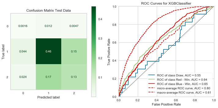
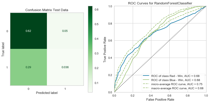
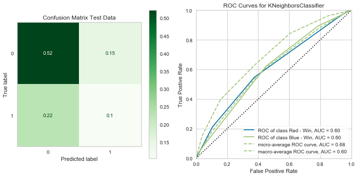
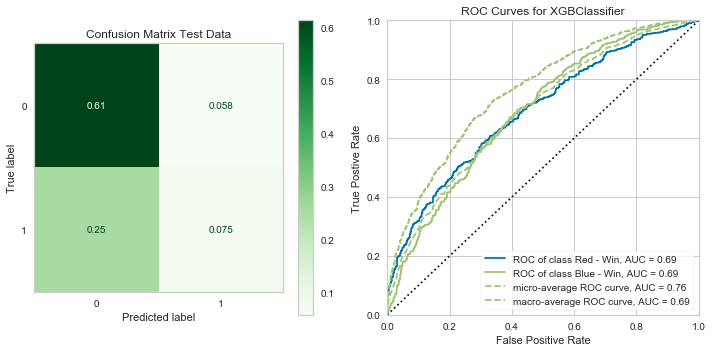
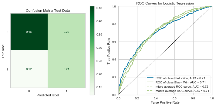
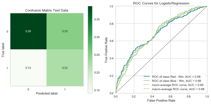
Not entirely what I expected. But it is clear that my model is failing to predict class 0 (Draw outcome). I am going to try my hand at a binary classification.
## Starting over and resetting target to only include fights with a winner
dummy_binary = pd.get_dummies(cat_df)
dummy_binary.drop(columns=['title_bout', 'Winner_Red'], inplace=True)
draws = dummy_binary[dummy_binary['Winner_Draw'] == 1].index
dummy_binary.drop(columns='Winner_Draw', index=draws, inplace=True)
dummy_binary.head().dataframe tbody tr th {
vertical-align: top;
}
.dataframe thead th {
text-align: right;
}
| Winner_Blue | weight_class_Bantamweight | weight_class_Catch Weight | weight_class_Featherweight | weight_class_Flyweight | weight_class_Heavyweight | weight_class_Light Heavyweight | weight_class_Lightweight | weight_class_Middleweight | weight_class_Open Weight | ... | B_Stance_Open Stance | B_Stance_Orthodox | B_Stance_Sideways | B_Stance_Southpaw | B_Stance_Switch | R_Stance_Open Stance | R_Stance_Orthodox | R_Stance_Sideways | R_Stance_Southpaw | R_Stance_Switch | |
|---|---|---|---|---|---|---|---|---|---|---|---|---|---|---|---|---|---|---|---|---|---|
| 0 | 0 | 1 | 0 | 0 | 0 | 0 | 0 | 0 | 0 | 0 | ... | 0 | 1 | 0 | 0 | 0 | 0 | 1 | 0 | 0 | 0 |
| 1 | 0 | 0 | 0 | 0 | 0 | 0 | 0 | 0 | 0 | 0 | ... | 0 | 1 | 0 | 0 | 0 | 0 | 0 | 0 | 1 | 0 |
| 2 | 0 | 0 | 0 | 0 | 0 | 0 | 0 | 1 | 0 | 0 | ... | 0 | 1 | 0 | 0 | 0 | 0 | 1 | 0 | 0 | 0 |
| 3 | 1 | 1 | 0 | 0 | 0 | 0 | 0 | 0 | 0 | 0 | ... | 0 | 0 | 0 | 0 | 1 | 0 | 1 | 0 | 0 | 0 |
| 4 | 1 | 0 | 0 | 0 | 0 | 1 | 0 | 0 | 0 | 0 | ... | 0 | 0 | 0 | 1 | 0 | 0 | 0 | 0 | 1 | 0 |
5 rows × 25 columns
## Putting it all together again
df_full_binary = pd.concat([df_fill.drop(columns=drop_cols), win_series, title_series], axis=1).copy()df_full_binary.drop(index=draws, inplace=True)
df_full_binary = pd.concat([df_full_binary, dummy_binary], axis=1)
#df_full_binary.head()## Train-test split
y_bin = df_full_binary['Winner_Blue'].copy()
X_bin = df_full_binary.drop(['Winner_Blue', 'Winner'], axis=1).copy()
X_train_bin, X_test_bin, y_train_bin, y_test_bin = train_test_split(X_bin, y_bin)print('Original Class Balance')
display(y_bin.value_counts(normalize=True))
print('y_train Class Balance')
display(y_train_bin.value_counts(normalize=True))
print('y_test Class Balance')
display(y_test_bin.value_counts(normalize=True))Original Class Balance
0 0.685635
1 0.314365
Name: Winner_Blue, dtype: float64
y_train Class Balance
0 0.690382
1 0.309618
Name: Winner_Blue, dtype: float64
y_test Class Balance
0 0.671406
1 0.328594
Name: Winner_Blue, dtype: float64
## Min max scale to help with varying values
scaler_bin = MinMaxScaler()
X_train_sca_bin = pd.DataFrame(scaler.fit_transform(X_train_bin), columns=X_train_bin.columns,
index=X_train_bin.index)
X_test_sca_bin = pd.DataFrame(scaler.transform(X_test_bin), columns=X_test_bin.columns,
index=X_test_bin.index)## Fix class imbalance
print('Original class distribution: \n')
print(y_train_bin.value_counts())
smote_bin = SMOTE()
X_trn_sca_resmp_bin, y_trn_resmp_bin = smote_bin.fit_sample(X_train_sca_bin, y_train_bin)
X_trn_sca_resmp_bin = pd.DataFrame(X_trn_sca_resmp_bin, columns=X_train_sca_bin.columns)
## Preview resampled class distribution
print('-----------------------------------------')
print('Resampled class distribution: \n')
print(pd.Series(y_trn_resmp_bin).value_counts()) Original class distribution:
0 2620
1 1175
Name: Winner_Blue, dtype: int64
-----------------------------------------
Resampled class distribution:
1 2620
0 2620
dtype: int64
tree_clf_bin = DecisionTreeClassifier(class_weight='balanced')
rf_clf_bin = RandomForestClassifier(class_weight='balanced')
log_clf_bin = LogisticRegression(C=1e9, class_weight='balanced', solver='liblinear')
knn_clf_bin = KNeighborsClassifier()
ada_clf_bin = AdaBoostClassifier()
grad_clf_bin = GradientBoostingClassifier()
xgb_clf_bin = xgb.XGBClassifier()mods_bin = [log_clf_bin, tree_clf_bin, rf_clf_bin, knn_clf_bin, ada_clf_bin, grad_clf_bin, xgb_clf_bin]
mod_labs_bin = ['log_clf_bin', 'tree_clf_bin', 'rf_clf_bin', 'knn_clf_bin', 'ada_clf_bin', 'grad_clf_bin', 'xgb_clf_bin']
t_bin = dlf.Timer()
labs_bin = ['Red - Win', 'Blue - Win']
times_bin = dlf.time_models(X_train_sca_bin, X_test_sca_bin, y_train_bin, y_test_bin, mods_bin, mod_labs_bin, t_bin, cls_lab=labs_bin)LogisticRegression(C=1000000000.0, class_weight='balanced', dual=False,
fit_intercept=True, intercept_scaling=1, l1_ratio=None,
max_iter=100, multi_class='auto', n_jobs=None, penalty='l2',
random_state=None, solver='liblinear', tol=0.0001, verbose=0,
warm_start=False)
Classification Report Test
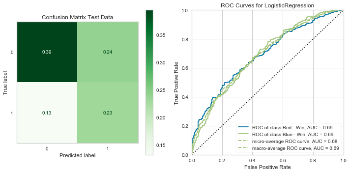
precision recall f1-score support
0 0.81 0.69 0.74 850
1 0.51 0.66 0.58 416
accuracy 0.68 1266
macro avg 0.66 0.68 0.66 1266
weighted avg 0.71 0.68 0.69 1266
---- Timer stopped at: 04/27/2020 - 09:24 PM ----
---- Time elasped: 0:00:01.476020 ----
DecisionTreeClassifier(ccp_alpha=0.0, class_weight='balanced', criterion='gini',
max_depth=None, max_features=None, max_leaf_nodes=None,
min_impurity_decrease=0.0, min_impurity_split=None,
min_samples_leaf=1, min_samples_split=2,
min_weight_fraction_leaf=0.0, presort='deprecated',
random_state=None, splitter='best')
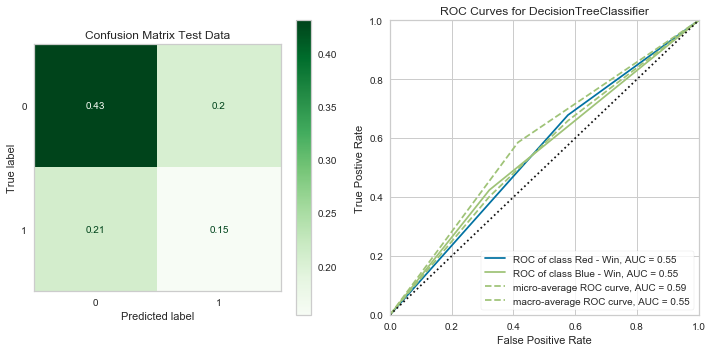
Classification Report Test
precision recall f1-score support
0 0.71 0.70 0.70 850
1 0.41 0.42 0.41 416
accuracy 0.61 1266
macro avg 0.56 0.56 0.56 1266
weighted avg 0.61 0.61 0.61 1266
---- Timer stopped at: 04/27/2020 - 09:24 PM ----
---- Time elasped: 0:00:01.048227 ----
RandomForestClassifier(bootstrap=True, ccp_alpha=0.0, class_weight='balanced',
criterion='gini', max_depth=None, max_features='auto',
max_leaf_nodes=None, max_samples=None,
min_impurity_decrease=0.0, min_impurity_split=None,
min_samples_leaf=1, min_samples_split=2,
min_weight_fraction_leaf=0.0, n_estimators=100,
n_jobs=None, oob_score=False, random_state=None,
verbose=0, warm_start=False)
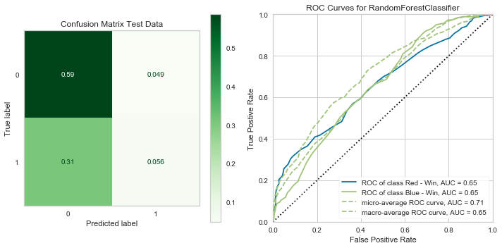
Classification Report Test
precision recall f1-score support
0 0.68 0.93 0.78 850
1 0.42 0.11 0.17 416
accuracy 0.66 1266
macro avg 0.55 0.52 0.48 1266
weighted avg 0.59 0.66 0.58 1266
---- Timer stopped at: 04/27/2020 - 09:24 PM ----
---- Time elasped: 0:00:03.333059 ----
KNeighborsClassifier(algorithm='auto', leaf_size=30, metric='minkowski',
metric_params=None, n_jobs=None, n_neighbors=5, p=2,
weights='uniform')
Classification Report Test
precision recall f1-score support
0 0.70 0.78 0.74 850
1 0.41 0.32 0.36 416
accuracy 0.63 1266
macro avg 0.56 0.55 0.55 1266
weighted avg 0.60 0.63 0.61 1266
---- Timer stopped at: 04/27/2020 - 09:24 PM ----
---- Time elasped: 0:00:12.550474 ----
AdaBoostClassifier(algorithm='SAMME.R', base_estimator=None, learning_rate=1.0,
n_estimators=50, random_state=None)
Classification Report Test
precision recall f1-score support
0 0.72 0.88 0.79 850
1 0.54 0.30 0.38 416
accuracy 0.69 1266
macro avg 0.63 0.59 0.59 1266
weighted avg 0.66 0.69 0.66 1266
---- Timer stopped at: 04/27/2020 - 09:24 PM ----
---- Time elasped: 0:00:02.401591 ----
GradientBoostingClassifier(ccp_alpha=0.0, criterion='friedman_mse', init=None,
learning_rate=0.1, loss='deviance', max_depth=3,
max_features=None, max_leaf_nodes=None,
min_impurity_decrease=0.0, min_impurity_split=None,
min_samples_leaf=1, min_samples_split=2,
min_weight_fraction_leaf=0.0, n_estimators=100,
n_iter_no_change=None, presort='deprecated',
random_state=None, subsample=1.0, tol=0.0001,
validation_fraction=0.1, verbose=0,
warm_start=False)
Classification Report Test
precision recall f1-score support
0 0.71 0.91 0.80 850
1 0.57 0.24 0.33 416
accuracy 0.69 1266
macro avg 0.64 0.57 0.57 1266
weighted avg 0.66 0.69 0.65 1266
---- Timer stopped at: 04/27/2020 - 09:24 PM ----
---- Time elasped: 0:00:07.875940 ----
XGBClassifier(base_score=0.5, booster='gbtree', colsample_bylevel=1,
colsample_bytree=1, gamma=0, learning_rate=0.1, max_delta_step=0,
max_depth=3, min_child_weight=1, missing=None, n_estimators=100,
n_jobs=1, nthread=None, objective='binary:logistic',
random_state=0, reg_alpha=0, reg_lambda=1, scale_pos_weight=1,
seed=None, silent=True, subsample=1)
Classification Report Test
precision recall f1-score support
0 0.71 0.91 0.80 850
1 0.56 0.23 0.32 416
accuracy 0.69 1266
macro avg 0.63 0.57 0.56 1266
weighted avg 0.66 0.69 0.64 1266
---- Timer stopped at: 04/27/2020 - 09:24 PM ----
---- Time elasped: 0:00:02.666879 ----
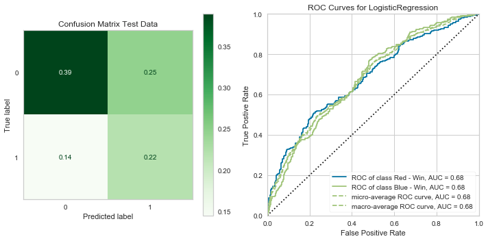
Pretty similar results to the multi-class models, hopefully running some grid searches will help.
## For reference
#rf_clf_bin = RandomForestClassifier(class_weight='balanced')
#tree_clf_bin = DecisionTreeClassifier(class_weight='balanced')tree_params_bin = {'criterion': ['gini', 'entropy'],
'min_samples_leaf': [3],
'max_depth': [10],
'max_features': [0.8, 0.5]}
tree_gridsrch_bin = dlf.grid_searcher(tree_clf_bin, tree_params_bin, X_trn_sca_resmp_bin,
X_test_sca_bin, y_trn_resmp_bin, y_test_bin, cv=3)---- Timer stopped at: 04/27/2020 - 09:27 PM ----
---- Time elasped: 0:00:03.375974 ----
Mean Training Score: 85.28%
Mean Test Score: 60.43%
Best Parameters:
{'criterion': 'entropy', 'max_depth': 10, 'max_features': 0.8, 'min_samples_leaf': 3}
log_params_bin = {'C': [1e12, 1e5, 1e2, 1],
'solver': ['liblinear', 'saga']}
log_gridsrch_bin = dlf.grid_searcher(log_clf_bin, log_params_bin, X_trn_sca_resmp_bin,
X_test_sca_bin, y_trn_resmp_bin, y_test_bin, cv=3)---- Timer stopped at: 04/27/2020 - 09:28 PM ----
---- Time elasped: 0:00:16.271521 ----
Mean Training Score: 70.18%
Mean Test Score: 67.69%
Best Parameters:
{'C': 100.0, 'solver': 'liblinear'}
log_params_bin2 = {'C': [1],
'solver': ['liblinear']}
log_gridsrch_bin2 = dlf.grid_searcher(log_clf_bin, log_params_bin2, X_trn_sca_resmp_bin,
X_test_sca_bin, y_trn_resmp_bin, y_test_bin, cv=3)---- Timer stopped at: 04/27/2020 - 09:28 PM ----
---- Time elasped: 0:00:00.531575 ----
Mean Training Score: 69.73%
Mean Test Score: 66.19%
Best Parameters:
{'C': 1, 'solver': 'liblinear'}
log_clf_bin_fin = LogisticRegression(C=1, class_weight='balanced', solver='liblinear')
mods_bin_fin = [log_clf_bin_fin]
mod_labs_bin_fin = ['log_clf_bin_fin']
t_bin_fin = dlf.Timer()
times_bin_fin = dlf.time_models(X_train_sca_bin, X_test_sca_bin, y_train_bin, y_test_bin, mods_bin_fin, mod_labs_bin_fin, t_bin_fin, cls_lab=labs_bin)LogisticRegression(C=1, class_weight='balanced', dual=False, fit_intercept=True,
intercept_scaling=1, l1_ratio=None, max_iter=100,
multi_class='auto', n_jobs=None, penalty='l2',
random_state=None, solver='liblinear', tol=0.0001, verbose=0,
warm_start=False)
Classification Report Test
precision recall f1-score support
0 0.79 0.68 0.73 850
1 0.49 0.63 0.55 416
accuracy 0.66 1266
macro avg 0.64 0.66 0.64 1266
weighted avg 0.69 0.66 0.67 1266
---- Timer stopped at: 04/27/2020 - 09:29 PM ----
---- Time elasped: 0:00:00.712094 ----
By using the logistic regression model and re-formatting the problem I was able to get an overall accuracy of 66%. Although not much better, I prefer this one due to the number of true positives it was able to generate comparatively.
My thoughts now are that maybe the use of fighters without a history could be holding my model back, because it is making a guess about something without a value in many of the possible attributes.
print(df.shape)
print(df_full_binary.shape)(5144, 140)
(5061, 162)
Here I dropped all of those avgs I filled previously
## Create a copy of the master and drop all of the rows with non-experienced
## fighters
df_fill_bin = df.copy()
df_fill_bin.dropna(subset=zero_fill_cols, inplace=True)## Quick helper to minimize code length
df_fill_bin = dlf.NA_handler_bin(df_fill_bin);Stance Distributions:
Orthodox 0.763011
Southpaw 0.202574
Switch 0.032457
Open Stance 0.001399
Sideways 0.000560
Name: B_Stance, dtype: float64
Orthodox 0.754479
Southpaw 0.214166
Switch 0.027996
Open Stance 0.003359
Name: R_Stance, dtype: float64
Stances:
['Orthodox', 'Switch', 'Southpaw', 'Open Stance', 'Sideways']
Stance Probabilities:
[7.63010632e-01 2.02574147e-01 3.24566312e-02 1.39899273e-03
5.59597090e-04]
Null Values Remaining:
4800 NaN
4814 NaN
Name: R_Reach_cms, dtype: float64
4800 NaN
4814 NaN
Name: B_Reach_cms, dtype: float64
Age Mean:
B_age 29.649220
R_age 29.940319
dtype: float64
Midpoint Age Mean:
29.79476976094046
<matplotlib.axes._subplots.AxesSubplot at 0x15474441828>
cat_df_bin_skim = df_fill_bin.select_dtypes(['object', 'bool']).copy()
dummy_binary_skim = pd.get_dummies(cat_df_bin_skim)
dummy_binary_skim.drop(columns=['title_bout', 'Winner_Red'], inplace=True)
draws_skim = dummy_binary_skim[dummy_binary_skim['Winner_Draw'] == 1].index
dummy_binary_skim.drop(columns='Winner_Draw', index=draws_skim, inplace=True)
print('Dummy Df columns:')
print(dummy_binary_skim.columns, '\n')
title_series_skim = cat_df_bin_skim['title_bout'].copy()
title_series_skim = title_series_skim.map(dict_title)
print('Title Bout Values:')
display(title_series_skim.head())Dummy Df columns:
Index(['Winner_Blue', 'weight_class_Bantamweight', 'weight_class_Catch Weight',
'weight_class_Featherweight', 'weight_class_Flyweight',
'weight_class_Heavyweight', 'weight_class_Light Heavyweight',
'weight_class_Lightweight', 'weight_class_Middleweight',
'weight_class_Open Weight', 'weight_class_Welterweight',
'weight_class_Women's Bantamweight',
'weight_class_Women's Featherweight', 'weight_class_Women's Flyweight',
'weight_class_Women's Strawweight', 'B_Stance_Open Stance',
'B_Stance_Orthodox', 'B_Stance_Sideways', 'B_Stance_Southpaw',
'B_Stance_Switch', 'R_Stance_Open Stance', 'R_Stance_Orthodox',
'R_Stance_Southpaw', 'R_Stance_Switch'],
dtype='object')
Title Bout Values:
0    1
1    1
2    0
3    0
4    0
Name: title_bout, dtype: int64
df_skim_binary = pd.concat([df_fill_bin.drop(columns=drop_cols), title_series_skim], axis=1).copy()df_skim_binary.drop(index=draws_skim, inplace=True)
df_skim_binary = pd.concat([df_skim_binary, dummy_binary_skim], axis=1)
print(df_skim_binary.shape)
df_skim_binary.head()(3592, 160)
.dataframe tbody tr th {
    vertical-align: top;
}

.dataframe thead th {
    text-align: right;
}
| no_of_rounds | B_current_lose_streak | B_current_win_streak | B_draw | B_avg_BODY_att | B_avg_BODY_landed | B_avg_CLINCH_att | B_avg_CLINCH_landed | B_avg_DISTANCE_att | B_avg_DISTANCE_landed | ... | weight_class_Women's Strawweight | B_Stance_Open Stance | B_Stance_Orthodox | B_Stance_Sideways | B_Stance_Southpaw | B_Stance_Switch | R_Stance_Open Stance | R_Stance_Orthodox | R_Stance_Southpaw | R_Stance_Switch | |
|---|---|---|---|---|---|---|---|---|---|---|---|---|---|---|---|---|---|---|---|---|---|
| 0 | 5 | 0.0 | 4.0 | 0.0 | 9.200000 | 6.000000 | 0.200000 | 0.000000 | 62.600000 | 20.600000 | ... | 0 | 0 | 1 | 0 | 0 | 0 | 0 | 1 | 0 | 0 |
| 1 | 5 | 0.0 | 3.0 | 0.0 | 14.600000 | 9.100000 | 11.800000 | 7.300000 | 124.700000 | 42.100000 | ... | 0 | 0 | 1 | 0 | 0 | 0 | 0 | 0 | 1 | 0 |
| 2 | 3 | 0.0 | 3.0 | 0.0 | 15.354839 | 11.322581 | 6.741935 | 4.387097 | 84.741935 | 38.580645 | ... | 0 | 0 | 1 | 0 | 0 | 0 | 0 | 1 | 0 | 0 |
| 3 | 3 | 0.0 | 4.0 | 0.0 | 17.000000 | 14.000000 | 13.750000 | 11.000000 | 109.500000 | 48.750000 | ... | 0 | 0 | 0 | 0 | 0 | 1 | 0 | 1 | 0 | 0 |
| 4 | 3 | 0.0 | 1.0 | 0.0 | 17.000000 | 14.500000 | 2.500000 | 2.000000 | 201.000000 | 59.500000 | ... | 0 | 0 | 0 | 0 | 1 | 0 | 0 | 0 | 1 | 0 |
5 rows × 160 columns
y_bin_skim = df_skim_binary['Winner_Blue'].copy()
X_bin_skim = df_skim_binary.drop(['Winner_Blue'], axis=1).copy()

X_train_bin_skim, X_test_bin_skim, y_train_bin_skim, y_test_bin_skim = train_test_split(X_bin_skim, y_bin_skim, test_size=0.2)X_bin_skim.columnsIndex(['no_of_rounds', 'B_current_lose_streak', 'B_current_win_streak',
'B_draw', 'B_avg_BODY_att', 'B_avg_BODY_landed', 'B_avg_CLINCH_att',
'B_avg_CLINCH_landed', 'B_avg_DISTANCE_att', 'B_avg_DISTANCE_landed',
...
'weight_class_Women's Strawweight', 'B_Stance_Open Stance',
'B_Stance_Orthodox', 'B_Stance_Sideways', 'B_Stance_Southpaw',
'B_Stance_Switch', 'R_Stance_Open Stance', 'R_Stance_Orthodox',
'R_Stance_Southpaw', 'R_Stance_Switch'],
dtype='object', length=159)
print('Original Class Balance')
display(y_bin_skim.value_counts(normalize=True))
print('y_train Class Balance')
display(y_train_bin_skim.value_counts(normalize=True))
print('y_test Class Balance')
display(y_test_bin_skim.value_counts(normalize=True))
Original Class Balance
0 0.662584
1 0.337416
Name: Winner_Blue, dtype: float64
y_train Class Balance
0 0.669335
1 0.330665
Name: Winner_Blue, dtype: float64
y_test Class Balance
0 0.635605
1 0.364395
Name: Winner_Blue, dtype: float64
scaler_bin_skim = MinMaxScaler()

X_train_sca_bin_skim = pd.DataFrame(scaler.fit_transform(X_train_bin_skim), columns=X_train_bin_skim.columns,
                           index=X_train_bin_skim.index)
X_test_sca_bin_skim = pd.DataFrame(scaler.transform(X_test_bin_skim), columns=X_test_bin_skim.columns,
index=X_test_bin_skim.index)print('Original class distribution: \n')
print(y_train_bin_skim.value_counts())
smote_bin_skim = SMOTE()
X_trn_sca_resmp_bin_skim, y_trn_resmp_bin_skim = smote_bin_skim.fit_sample(X_train_sca_bin_skim, y_train_bin_skim)
X_trn_sca_resmp_bin_skim = pd.DataFrame(X_trn_sca_resmp_bin_skim, columns=X_train_sca_bin_skim.columns)
# Preview synthetic sample class distribution
print('-----------------------------------------')
print('Resampled class distribution: \n')
print(pd.Series(y_trn_resmp_bin_skim).value_counts()) Original class distribution:
0 1923
1 950
Name: Winner_Blue, dtype: int64
-----------------------------------------
Resampled class distribution:
1 1923
0 1923
dtype: int64
tree_clf_bin2 = DecisionTreeClassifier(class_weight='balanced')
rf_clf_bin2 = RandomForestClassifier(class_weight='balanced')
log_clf_bin2 = LogisticRegression(class_weight='balanced', solver='liblinear')
knn_clf_bin2 = KNeighborsClassifier()
ada_clf_bin2 = AdaBoostClassifier()
grad_clf_bin2 = GradientBoostingClassifier()
xgb_clf_bin2 = xgb.XGBClassifier()
mods_bin2 = [log_clf_bin2, tree_clf_bin2, rf_clf_bin2, knn_clf_bin2, ada_clf_bin2, grad_clf_bin2, xgb_clf_bin2]
mod_labs_bin2 = ['log_clf_bin2', 'tree_clf_bin2', 'rf_clf_bin2', 'knn_clf_bin2', 'ada_clf_bin2', 'grad_clf_bin2', 'xgb_clf_bin2']
t_bin2 = dlf.Timer()
labs_bin = ['Red - Win', 'Blue - Win']
times_bin2 = dlf.time_models(X_train_sca_bin_skim, X_test_sca_bin_skim, y_train_bin_skim, y_test_bin_skim, mods_bin2, mod_labs_bin2, t_bin2, cls_lab=labs_bin)LogisticRegression(C=1.0, class_weight='balanced', dual=False,
fit_intercept=True, intercept_scaling=1, l1_ratio=None,
max_iter=100, multi_class='auto', n_jobs=None, penalty='l2',
random_state=None, solver='liblinear', tol=0.0001, verbose=0,
warm_start=False)
Classification Report Test
precision recall f1-score support
0 0.75 0.62 0.68 457
1 0.49 0.64 0.55 262
accuracy 0.63 719
macro avg 0.62 0.63 0.62 719
weighted avg 0.66 0.63 0.63 719
---- Timer stopped at: 04/27/2020 - 09:47 PM ----
---- Time elasped: 0:00:00.705115 ----


DecisionTreeClassifier(ccp_alpha=0.0, class_weight='balanced', criterion='gini',
                       max_depth=None, max_features=None, max_leaf_nodes=None,
                       min_impurity_decrease=0.0, min_impurity_split=None,
                       min_samples_leaf=1, min_samples_split=2,
                       min_weight_fraction_leaf=0.0, presort='deprecated',
                       random_state=None, splitter='best')


Classification Report Test
              precision    recall  f1-score   support

           0       0.67      0.68      0.68       457
           1       0.43      0.42      0.43       262

    accuracy                           0.59       719
   macro avg       0.55      0.55      0.55       719
weighted avg       0.58      0.59      0.58       719
---- Timer stopped at: 04/27/2020 - 09:47 PM ----
---- Time elasped: 0:00:00.896603 ----


RandomForestClassifier(bootstrap=True, ccp_alpha=0.0, class_weight='balanced',
                       criterion='gini', max_depth=None, max_features='auto',
                       max_leaf_nodes=None, max_samples=None,
                       min_impurity_decrease=0.0, min_impurity_split=None,
                       min_samples_leaf=1, min_samples_split=2,
                       min_weight_fraction_leaf=0.0, n_estimators=100,
                       n_jobs=None, oob_score=False, random_state=None,
                       verbose=0, warm_start=False)


Classification Report Test
              precision    recall  f1-score   support

           0       0.66      0.92      0.77       457
           1       0.53      0.15      0.24       262

    accuracy                           0.64       719
   macro avg       0.59      0.54      0.50       719
weighted avg       0.61      0.64      0.57       719
---- Timer stopped at: 04/27/2020 - 09:47 PM ----
---- Time elasped: 0:00:02.875342 ----


KNeighborsClassifier(algorithm='auto', leaf_size=30, metric='minkowski',
                     metric_params=None, n_jobs=None, n_neighbors=5, p=2,
                     weights='uniform')


Classification Report Test
              precision    recall  f1-score   support

           0       0.67      0.81      0.73       457
           1       0.48      0.31      0.38       262

    accuracy                           0.62       719
   macro avg       0.57      0.56      0.55       719
weighted avg       0.60      0.62      0.60       719
---- Timer stopped at: 04/27/2020 - 09:47 PM ----
---- Time elasped: 0:00:07.565786 ----


AdaBoostClassifier(algorithm='SAMME.R', base_estimator=None, learning_rate=1.0,
                   n_estimators=50, random_state=None)


Classification Report Test
              precision    recall  f1-score   support

           0       0.68      0.81      0.74       457
           1       0.51      0.35      0.41       262

    accuracy                           0.64       719
   macro avg       0.60      0.58      0.58       719
weighted avg       0.62      0.64      0.62       719
---- Timer stopped at: 04/27/2020 - 09:47 PM ----
---- Time elasped: 0:00:02.303829 ----


GradientBoostingClassifier(ccp_alpha=0.0, criterion='friedman_mse', init=None,
                           learning_rate=0.1, loss='deviance', max_depth=3,
                           max_features=None, max_leaf_nodes=None,
                           min_impurity_decrease=0.0, min_impurity_split=None,
                           min_samples_leaf=1, min_samples_split=2,
                           min_weight_fraction_leaf=0.0, n_estimators=100,
                           n_iter_no_change=None, presort='deprecated',
                           random_state=None, subsample=1.0, tol=0.0001,
                           validation_fraction=0.1, verbose=0,
                           warm_start=False)


Classification Report Test
              precision    recall  f1-score   support

           0       0.67      0.89      0.77       457
           1       0.56      0.24      0.34       262

    accuracy                           0.65       719
   macro avg       0.61      0.57      0.55       719
weighted avg       0.63      0.65      0.61       719
---- Timer stopped at: 04/27/2020 - 09:47 PM ----
---- Time elasped: 0:00:07.590721 ----


XGBClassifier(base_score=0.5, booster='gbtree', colsample_bylevel=1,
              colsample_bytree=1, gamma=0, learning_rate=0.1, max_delta_step=0,
              max_depth=3, min_child_weight=1, missing=None, n_estimators=100,
              n_jobs=1, nthread=None, objective='binary:logistic',
              random_state=0, reg_alpha=0, reg_lambda=1, scale_pos_weight=1,
              seed=None, silent=True, subsample=1)


Classification Report Test
              precision    recall  f1-score   support

           0       0.68      0.88      0.76       457
           1       0.55      0.27      0.36       262

    accuracy                           0.66       719
   macro avg       0.62      0.57      0.56       719
weighted avg       0.63      0.66      0.62       719
---- Timer stopped at: 04/27/2020 - 09:47 PM ----
---- Time elasped: 0:00:02.228032 ----
#ada_clf_bin2 = AdaBoostClassifier()
#log_clf_bin2 = LogisticRegression(class_weight='balanced', solver='liblinear')
log_params_bin_skim = {'C': [0.5, 1e10, 1e5],
'solver': ['liblinear', 'saga']}
log_gridsrch_bin_skim = dlf.grid_searcher(log_clf_bin2, log_params_bin_skim, X_trn_sca_resmp_bin_skim,
X_test_sca_bin_skim, y_trn_resmp_bin_skim, y_test_bin_skim, cv=3)---- Timer stopped at: 04/27/2020 - 09:49 PM ----
---- Time elasped: 0:00:13.517857 ----
Mean Training Score: 70.41%
Mean Test Score: 60.92%
Best Parameters:
{'C': 10000000000.0, 'solver': 'liblinear'}
log_params_bin_skim2 = {'C': [10],
'solver': ['liblinear', 'saga']}
log_gridsrch_bin_skim2 = dlf.grid_searcher(log_clf_bin2, log_params_bin_skim2, X_trn_sca_resmp_bin_skim,
X_test_sca_bin_skim, y_trn_resmp_bin_skim, y_test_bin_skim, cv=3)---- Timer stopped at: 04/27/2020 - 09:49 PM ----
---- Time elasped: 0:00:02.659925 ----
Mean Training Score: 70.57%
Mean Test Score: 60.92%
Best Parameters:
{'C': 10, 'solver': 'liblinear'}
ada_params_bin_skim = {'n_estimators': [100],
'learning_rate': [0.1, 0.175],
'base_estimator': [LogisticRegression(C=10, solver='saga')]}
ada_gridsrch_bin_skim = dlf.grid_searcher(ada_clf_bin2, ada_params_bin_skim, X_trn_sca_resmp_bin_skim,
X_test_sca_bin_skim, y_trn_resmp_bin_skim, y_test_bin_skim, cv=3)---- Timer stopped at: 04/27/2020 - 09:56 PM ----
---- Time elasped: 0:06:59.069704 ----
Mean Training Score: 64.85%
Mean Test Score: 62.87%
Best Parameters:
{'base_estimator': LogisticRegression(C=10, class_weight=None, dual=False, fit_intercept=True,
intercept_scaling=1, l1_ratio=None, max_iter=100,
multi_class='auto', n_jobs=None, penalty='l2',
random_state=None, solver='saga', tol=0.0001, verbose=0,
warm_start=False), 'learning_rate': 0.175, 'n_estimators': 100}
ada_params_bin_skim2 = {'n_estimators': [1000],
'learning_rate': [0.175],
'base_estimator': [LogisticRegression(C=100000, solver='liblinear')]}
ada_gridsrch_bin_skim2 = dlf.grid_searcher(ada_clf_bin2, ada_params_bin_skim2, X_trn_sca_resmp_bin_skim,
X_test_sca_bin_skim, y_trn_resmp_bin_skim, y_test_bin_skim, cv=3)---- Timer stopped at: 04/27/2020 - 10:04 PM ----
---- Time elasped: 0:07:24.547366 ----
Mean Training Score: 70.58%
Mean Test Score: 60.36%
Best Parameters:
{'base_estimator': LogisticRegression(C=100000, class_weight=None, dual=False, fit_intercept=True,
intercept_scaling=1, l1_ratio=None, max_iter=100,
multi_class='auto', n_jobs=None, penalty='l2',
random_state=None, solver='liblinear', tol=0.0001, verbose=0,
warm_start=False), 'learning_rate': 0.175, 'n_estimators': 1000}
log_skim1 = log_gridsrch_bin_skim.best_estimator_
log_skim2 = log_gridsrch_bin_skim2.best_estimator_
ada_skim = ada_gridsrch_bin_skim2.best_estimator_mods_skim_fin = [log_skim1, log_skim2, ada_skim]
mod_labs_skim_fin = ['log_skim1', 'log_skim2', 'ada_skim']
t_skim_fin = dlf.Timer()
times_skim_fin = dlf.time_models(X_trn_sca_resmp_bin_skim, X_test_sca_bin_skim, y_trn_resmp_bin_skim, y_test_bin_skim, mods_skim_fin, mod_labs_skim_fin, t_skim_fin, cls_lab=labs_bin)LogisticRegression(C=10000000000.0, class_weight='balanced', dual=False,
fit_intercept=True, intercept_scaling=1, l1_ratio=None,
max_iter=100, multi_class='auto', n_jobs=None, penalty='l2',
random_state=None, solver='liblinear', tol=0.0001, verbose=0,
warm_start=False)
Classification Report Test
precision recall f1-score support
0 0.73 0.61 0.66 457
1 0.47 0.61 0.53 262
accuracy 0.61 719
macro avg 0.60 0.61 0.60 719
weighted avg 0.64 0.61 0.62 719
---- Timer stopped at: 04/27/2020 - 10:05 PM ----
---- Time elasped: 0:00:02.478348 ----
LogisticRegression(C=10, class_weight='balanced', dual=False,
fit_intercept=True, intercept_scaling=1, l1_ratio=None,
max_iter=100, multi_class='auto', n_jobs=None, penalty='l2',
random_state=None, solver='liblinear', tol=0.0001, verbose=0,
warm_start=False)
Classification Report Test
precision recall f1-score support
0 0.73 0.61 0.67 457
1 0.47 0.60 0.53 262
accuracy 0.61 719
macro avg 0.60 0.61 0.60 719
weighted avg 0.64 0.61 0.62 719
---- Timer stopped at: 04/27/2020 - 10:05 PM ----
---- Time elasped: 0:00:00.954477 ----
AdaBoostClassifier(algorithm='SAMME.R',
base_estimator=LogisticRegression(C=100000,
class_weight=None,
dual=False,
fit_intercept=True,
intercept_scaling=1,
l1_ratio=None,
max_iter=100,
multi_class='auto',
n_jobs=None, penalty='l2',
random_state=None,
solver='liblinear',
tol=0.0001, verbose=0,
warm_start=False),
learning_rate=0.175, n_estimators=1000, random_state=None)
Classification Report Test
precision recall f1-score support
0 0.72 0.61 0.66 457
1 0.47 0.59 0.52 262
accuracy 0.60 719
macro avg 0.59 0.60 0.59 719
weighted avg 0.63 0.60 0.61 719
---- Timer stopped at: 04/27/2020 - 10:08 PM ----
---- Time elasped: 0:03:04.412768 ----
It has actually lowered the accuracy! I will stick with my 2nd model moving forward.
Throughout the duration of this project, I have created and tuned three models looking at the data three different ways. My results and correspsonding model parameters are as follows:
#multi_y_trn, multi_y_te = fit_n_pred(xgb_fin, X_trn_sca_resmp, X_test_sca, y_trn_resmp)dlf.summarize_model(xgb_fin, X_trn_sca_resmp, X_test_sca, y_trn_resmp, y_test, tree=True)XGBClassifier(base_score=0.5, booster='gbtree', colsample_bylevel=1,
colsample_bytree=1, gamma=0, learning_rate=0.05, max_delta_step=0,
max_depth=2, min_child_weight=1, missing=None, n_estimators=50,
n_jobs=1, nthread=None, num_class=3, objective='multi:softprob',
random_state=0, reg_alpha=0, reg_lambda=1, scale_pos_weight=1,
seed=None, silent=True, subsample=1)
Classification Report:
precision recall f1-score support
0 0.02 0.09 0.04 23
1 0.72 0.71 0.71 845
2 0.46 0.41 0.44 418
accuracy 0.60 1286
macro avg 0.40 0.40 0.40 1286
weighted avg 0.63 0.60 0.61 1286
#y_hat_trn_bin, y_hat_te_bin = fit_n_pred(log_clf_bin_fin, X_trn_sca_resmp_bin, X_test_sca_bin, y_trn_resmp_bin)dlf.summarize_model(log_clf_bin_fin, X_trn_sca_resmp_bin, X_test_sca_bin, y_trn_resmp_bin, y_test_bin)LogisticRegression(C=1, class_weight='balanced', dual=False, fit_intercept=True,
intercept_scaling=1, l1_ratio=None, max_iter=100,
multi_class='auto', n_jobs=None, penalty='l2',
random_state=None, solver='liblinear', tol=0.0001, verbose=0,
warm_start=False)
Classification Report:
precision recall f1-score support
0 0.78 0.69 0.73 850
1 0.49 0.61 0.54 416
accuracy 0.66 1266
macro avg 0.64 0.65 0.64 1266
weighted avg 0.69 0.66 0.67 1266
bin_full_test_probs = log_clf_bin_fin.predict_proba(X_test_sca_bin)
bin_full_test_probsarray([[0.35900333, 0.64099667],
[0.45309112, 0.54690888],
[0.78566549, 0.21433451],
...,
[0.5289652 , 0.4710348 ],
[0.57125872, 0.42874128],
[0.86817068, 0.13182932]])
#y_hat_trn_skim, y_hat_te_skim = fit_n_pred(log_skim1, X_train_sca_bin_skim, X_test_sca_bin_skim, y_train_bin_skim)dlf.summarize_model(log_skim1, X_trn_sca_resmp_bin_skim, X_test_sca_bin_skim, y_trn_resmp_bin_skim, y_test_bin_skim)LogisticRegression(C=10000000000.0, class_weight='balanced', dual=False,
fit_intercept=True, intercept_scaling=1, l1_ratio=None,
max_iter=100, multi_class='auto', n_jobs=None, penalty='l2',
random_state=None, solver='liblinear', tol=0.0001, verbose=0,
warm_start=False)
Classification Report:
precision recall f1-score support
0 0.73 0.61 0.66 457
1 0.47 0.61 0.53 262
accuracy 0.61 719
macro avg 0.60 0.61 0.60 719
weighted avg 0.64 0.61 0.62 719
bin_skim_test_probs = log_skim1.predict_proba(X_test_sca_bin_skim)
bin_skim_test_probsarray([[0.233598 , 0.766402 ],
[0.37351678, 0.62648322],
[0.64074403, 0.35925597],
...,
[0.89681032, 0.10318968],
[0.63998927, 0.36001073],
[0.70465062, 0.29534938]])
Given these results, I would recommend using one of the two binary classification models to make their predicitions. Out of the two, I recommend the model trained on data containing 1st time fighters
log_clf_bin_fin, as it has already seen data as such and over time with further development, be able to make a better prediction if fed that data.
The reasoning behind choosing this model is for its purpose: to allow interested parties to have a probability value associated with any given fighter to win the match. Although 66% overall accuracy is not high, this model recieved this score by correctly guessing over both classes (46%, 20%); whereas other modeling attempts correctly guessed one class ~65% right while missing almost all of guesses at the other.
As for the multi-class model, being unable to predict a draw at all is something that may require more data preprocessing or a different modeling strategy. Looking at the confusion matrix for it, the model clearly only predicted actual wins by either corner, which is why I decided to drop that class entirely.
If these models were to be used in any capacity, I can tailor the input features to whatever is necessary. As-is, I would expect it to be run using the same information scraped from ufcstats.com, but could always be altered to accept different subsets of features.
Additionally, combat sports by nature are very volatile when it comes to determining a winner. There are numerous ways to "get lucky" and steal a win, or to simply be in bad shape. There are intangibles such as "having heart" or a "strong chin" that would be difficult to quantify. In addition, important information such as fighting styles or what training camp they fight for could prove to be valuable to my model. Otherwise, given more time I would like to play more with what attributes I can add (or remove) in order to inch my accuracy higher.
