Tools for time-frequency analysis of noisy time series. The accompanying manuscript "Optimal time frequency analysis for biological data - pyBOAT" can be found here. For help, questions or comments please join the official chat at gitter or write an email to gregor.moenke@esi-frankfurt.de.
- Optimal sinc filter
- Fourier analysis
- Wavelet analysis
- Ridge detection
- Phase extraction
- Amplitude estimation
- Synthetic signal generator
- Ensemble statistics
pyBOAT is written in Python and therefore requires Python to be present on the system. An easy way to install a cross-platform scientfic Python environment is to use the freely availabe Anaconda Distribution. Installation instructions can be found here: https://docs.anaconda.com/anaconda/install/, a Python 3.x version is needed.
Once the Anaconda installation is complete, starting up the Anaconda Navigator
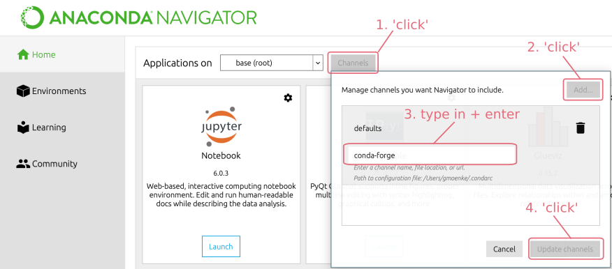
will show an interface like this:
First clicking on Channels and then on Add... will open an input field.
Type conda-forge into it and
confirm with the ⏎ enter key. Now after hitting Update channels, the
community packages hosted on the conda-forge channel will become available. As pyBOAT
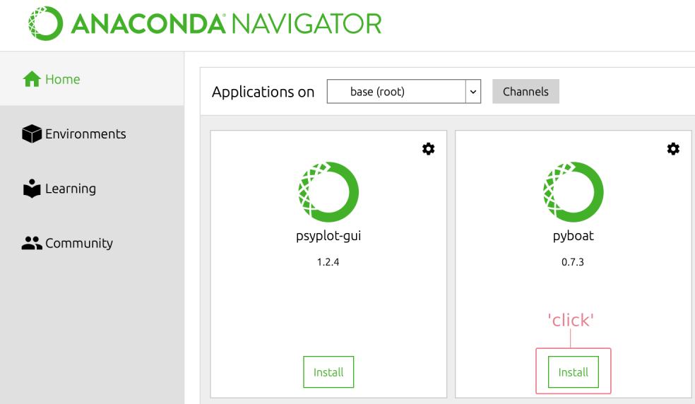
is also a Navigator App, it will now (along with other apps) show up in the main Navigator window:
Finally hitting Install will download and install pyBOAT. Thereafter,
pyBOAT can be started by simply clicking on Launch inside the Navigator.
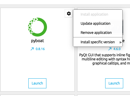
In case you see a little blue arrow next to the version number, this means an update is available. Clicking on the cogwheel icon in the upper right corner allows to run the update and install the latest version of pyBOAT.
For this, the download and installation of miniconda
is sufficient. Once conda is available on the commandline, typing
conda config --add channels conda-forge
will add the conda-forge channel to your conda. pyBOAT can then be installed with:
conda install pyboat
Now typing pyboat into the commandline will launch the GUI, and the pyboat
module is available for your Python environment.
pyBOAT is listed on the Python Package Index (PyPI)
and can be directly installed using pip. In case you don't have/want Anaconda,
see here for install instructions for pip itself: https://pip.pypa.io/en/stable/installing/.
To install pyboat simply type
pip install pyboat
into the command line. This makes the pyboat Python module available for import.
The graphical user interface (GUI) can be started by typing
pyboat
into the command line.
For running directly from the source, see also this document
Almost every input field and checkbox has a tool tip attached for quick reference.
In general pyBOAT expects tabular data, with each column
representing a signal. Just open your saved time-series data by using Open
from the (small) main window. Supported input formats are:
.xls, .xlsx, .csv, .tsv and .txt . For other file
extensions, white space separation of the data is assumed.
Please see examples of the supported formats in the
example_data directory of this repository.
In case you want to interpolate missing data or you want to define your own
separator, the Import.. button will spawn a menu with further options.
After successful import, you can simply click on the table representing
your data to select a specific time-series in the DataViewer.
Alternatively, select a specific time-series from the drop-down menu in the upper left.
To get the correct numbers/units you can change the Sampling Interval
and Time Unit name in the top line of the DataViewer.
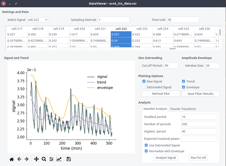
The general layout of the DataViewer to set up the analysis is shown here:
The featured sinc-detrending is an optimal high-pass filter and removes low frequencies (high periods)
from the signal via a sharp cut-off-period. Details of the implementation can be found at
The Scientist and Engineer's Guide to Digital Signal Processing.
Check the Trend and/or Detrended Signal checkbox(es)
and click Refresh Plot
to see the effect of the filter on the selected time series.
If there is a strong trend in the amplitudes alone, for example a slow decay, pyBOAT offers
a simple sliding-window operation to estimate this envelope. The Window Size
controls the time-window in which each amplitude is estimated.
Check the Envelope checkbox and click Refresh Plot
to see the detected envelope. When running the
Wavelet analysis, there is an option Normalize with Envelope to remove it
from the signal.
Set the parameters for the Wavelet Analysis in the lower right:
| Input Field | Meaning |
|---|---|
| Smallest Period | Lower period bound (Nyquist limit built-in) |
| Number of Periods | Resolution of the transform or number of convolutions |
| Highest Period | Upper period bound Should not exceed observation time |
| Expected maximal power | Upper bound for the colormap indicating the Wavelet power normalized to white noise |
Leave the Use the detrended signal box checked if you want to use the sinc-detrending.
Analyze Signal will perform the Wavelet transform of the selected signal.
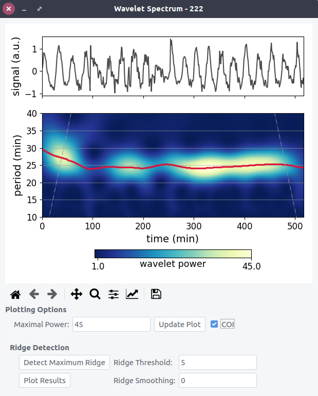
The input signal for the Wavelet analysis and the resulting 2d-power-spectrum are shown with aligned time axis.
The y-axis indicates the periods(frequencies) selected for analysis.
Bright areas indicate a high Wavelet power around this period(frequency) at that time of the signal. Some synthetic signals
for demonstrational purposes can be found in /example_data/synth_signal.csv.
Set a new Maximal Power and hit Update Plot to rescale the heatmap if needed.
The cone of influence (COI) can be plotted on top of the spectrum by checking the respective box.
To extract intantaneous frequency and associated phase, a 1d-ridge (a profile) has to be traced through the 2d-power spectrum:
This maps one frequency (or period) to one time point.
The simplest way is to connect all time-consecutive power-maxima. This is what
Detect Maximum Ridge does. This works well for all of the examples found in
/data_examples/synth_signal.csv.
To exclude parts of the spectrum whith
low Wavelet power, indicating that no oscillations wihtin the chosen period(frequency)
range are present at that time, set a Ridge Threshold. The actual ridge is indicated as a
red line in spectrum plot, note that no default ridge is shown in a fresh
Wavelet Spectrum window. For a quick check hit the Detect Maximum Ridge button.
You can also smooth the ridge if needed.
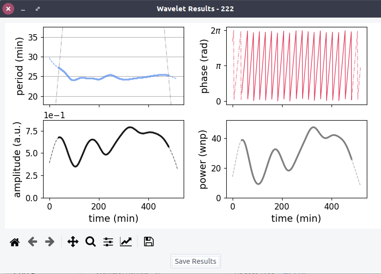
Once it is found, the complex Wavelet transform can be evaluated along
that ridge yielding a complex time series:
Plot Results will then show the extracted
instantaneous periods(frequencies), the phase and power profile along the ridge:


