Create virtual environment:
python3 -m venv env
On Mac or Linux run:
source env/bin/activate
On Windows run:
\Scripts\activate.bat
Install dependencies:
python3 -m pip install -r requirements.txt
Run the program:
python3 face_detection.py
We detect faces in face_detection.py using OpenCV and LBP cascades.
The face positions, along with their timestamps, are stored for
calculation.
The BPM calculation takes advantage of the periodicity of a head to calculate a frequency. The data processing can be split into four parts: (1) sampling, (2) velocity projection, (3) smoothing, and (4) curve fitting.
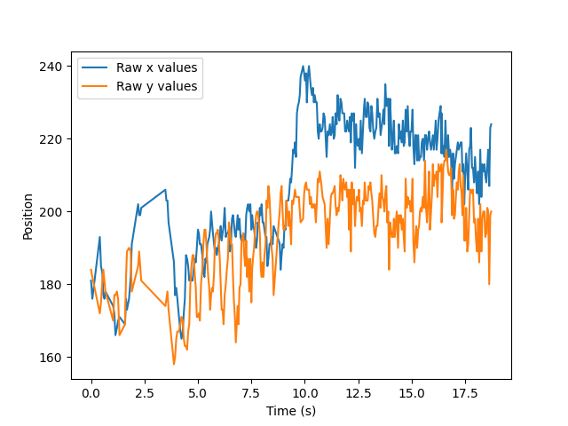
Rather than trying to determine the frequency of the data using the total aggregated data or the most recent data points, we randomly sample chunks of the data recorded. This is because some areas of the data may look may be far more periodic than others. In the figure below, the 4-8 second time frame is a much better candidate for fitting a sinusoidal curve than the most recent time frame is:
After randomly sampling chunks of the raw data, we follow the following steps for all samples.
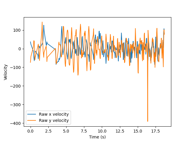
Head bops can be characterized by the head's position in space, but due to possible drifts in the actual position (like that shown in the above figure), the velocity is a more stable metric from which to determine the song's BPM. For periodic motion, a drift in position translates simply to a change in amplitude for some periods. The below figure shows the velocities for the same position data as shown above.
Since the timestamps may be irregular, these are calculated by using an average of the forward and backward one-sided derivatives, which converges to the centered-difference formula in the case that both timesteps are equal.
We calculate the song's BPM using a sinusoidal fit, so we ultimately would like a one-dimensional time series. Since most head bopping is (roughly) vertical, we use the y-velocity.
The above data shows excellent periodicity in the 4-8 second time window for the y-velocity. However, this may not always be the case. Bopping may look different from person to person and even song to song. So, we also calculate velocity along some average axis which we'll call the "bop vector." This is calculated by performing a linear fit on the sample positions and calculating a vector in the direction of the fit's slope. We then project the head's velocity at each timestep onto this bop vector.
There are several possible sources of error when projecting the velocities along the bop vector, so for some samples the y-data (which is equivalent to a vertical bop vector projection) may be better for calculating the BPM. We consider both possibilities by calculating a BPM for both sets of data and taking the one with less error.
We have a couple options for smoothing our data, a simple single moving
average
and a double exponentially-weighted moving average.
by default the double exponential smoothing is used because it captures
trends well. However, both work well.
We fit the data using a generalized sine function:
where
is the angular frequency of the function. We perform this
fit for both one-dimensional velocities calculated over all samples and
take the one with least squared error in the angular frequency
parameter, which is found by taking the corresponding diagonal element
of the covariance matrix returned by the fit.
To calculate the BPM, we convert the best fit's angular frequency to a
temporal frequency by simply dividing by . Finally, we convert this
per-second frequency to per-minute, giving the BPM.

