This repository contains the PyTorch Implementation of SubSpectralNets introduced in the following paper:
SubSpectralNet - Using Sub-Spectrogram based Convolutional Neural Networks for Acoustic Scene Classification (Accepted in ICASSP 2019)
Sai Samarth R Phaye, Emmanouil Benetos, and Ye Wang.
Click here for the presentation!
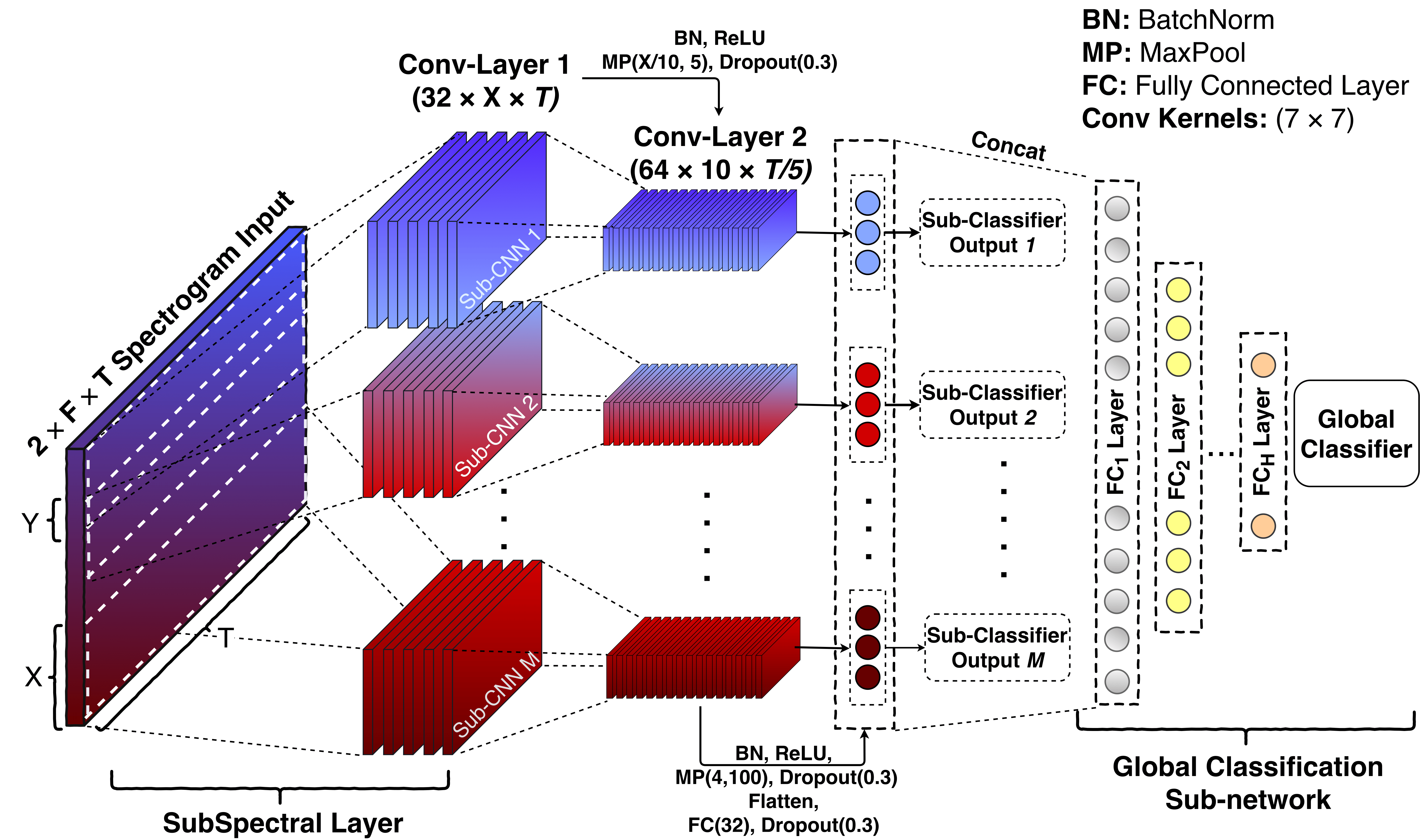
We introduce a novel approach of using spectrograms in Convolutional Neural Networks in the context of acoustic scene classification. First, we show from the statistical analysis that some specific bands of mel-spectrograms carry discriminative information than other bands, which is specific to every soundscape. From the inferences taken by this, we propose SubSpectralNets in which we first design a new convolutional layer that splits the time-frequency features into sub-spectrograms, then merges the band-level features on a later stage for the global classification. The effectiveness of SubSpectralNet is demonstrated by a relative improvement of +14% accuracy over the DCASE 2018 baseline model. The detailed architecture of SubSpectralNet is shown below.
If you have any queries regarding the code, please contact us on the following email: phaye.samarth@gmail.com (Sai Samarth R Phaye)
Following are the steps to follow for using this implementation:
Before anything, it is expected that you download and extract the DCASE 2018 ASC Development Dataset. You should obtain a folder named "TUT-urban-acoustic-scenes-2018-development", which contains various subfolders like "audio", "evaluation_setup" etc. Once you get this folder, following are the steps to execute the code:
Step 1. Clone the repository to local
git clone https://github.com/ssrp/SubSpectralNet-PyTorch.git SubSpectralNets
cd SubSpectralNets/code
Step 2. Install the prerequisites
pip install -r requirements.txt
Step 3. Train a SubSpectralNet
Train with default settings:
python main.py --root-dir <location_of_dataset>/TUT-urban-acoustic-scenes-2018-development/
For more settings, the code is well-commented and it's easy to change the parameters looking at the comments.
You should be able to see the losses for every iteration on the console. Additionally, you could also visualize the losses on TensorBoard by creating a tensorboard session using the following command (run on a new console, in the same directory):
tensorboard --logdir=.
For your convenience, there is one log file in the code/tensorboard-logs directory.
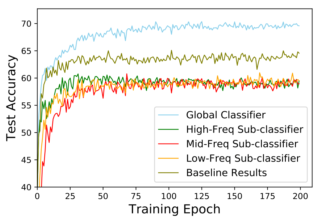
The statistical results of the network are shared in Section 4 of the paper. Following is the accuracy curve obtained after training the model on 40 mel-bin magnitude spectrograms, 20 sub-spectrogram size and 10 mel-bin hop-size (72.18%, average-best accuracy in three runs).

