#SCell user guide
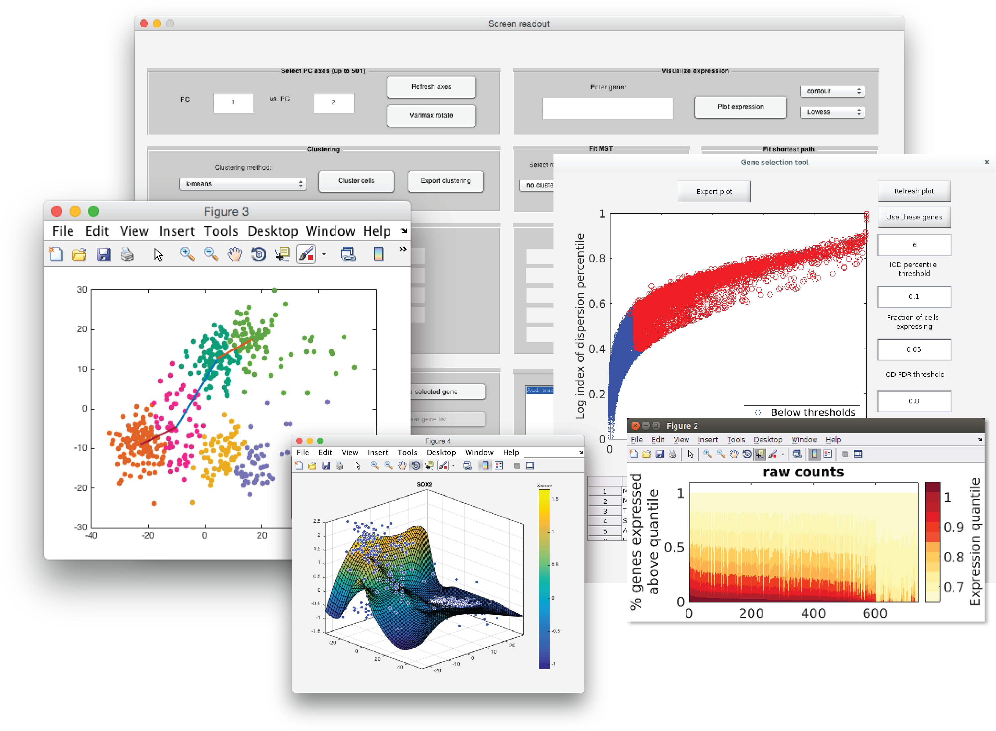
SCell is an integrated software tool for quality filtering, normalization, feature selection, iterative dimensionality reduction, clustering and the estimation of gene-expression gradients from large ensembles of single-cell RNA-seq datasets. SCell is open source, and implemented with an intuitive graphical interface.
Binary executables for Windows, MacOS and Linux are available at http://sourceforge.net/projects/scell, source code and pre-processing scripts are available from https://github.com/diazlab/SCell. If you use this software for your research, please cite: Aaron Diaz, Siyuan J. Liu, Carmen Sandoval, Alex Pollen, Tom J. Nowakowski, Daniel A. Lim, Arnold Kriegstein. SCell: integrated analysis of single-cell RNA-seq data. Bioinformatics. 2016. doi: 10.1093/bioinformatics/btw201
- Installation
- Load data and metadata
- Quality control & outlier filtering
- Gene panel selection and normalization
- Dimensionality reduction and PCA
- Visualize gene expression across cells
- Clustering
- Fit a minimum-spanning tree or minimum-cost path
- Iterative PCA
- Save and load sessions
- Preprocessing scripts
SCell runs under 64bit Mac OSX, Windows, and Linux. Start by downloading the appropriate installation package
from:
https://sourceforge.net/projects/scell/. Files that end in _web will have a smaller initial download, but will download more files during installation. Those without the _web ending have everything needed already bundled. Once downloaded double click the installer and follow the on-screen instructions. To invoke the Windows or MacOS executables click their icons, to invoke from the Linux or MacOS command line execute run_SCell.sh /path/to/matlab/runtime. If you want SCell to call preseq to estimate marginal return, you can install preseq here.
SCell is released under the GNU General Public License: http://www.gnu.org/licenses/. The SCell source code can be obtained from https://github.com/diazlab/scell.
SCell accepts as input a matrix of raw gene counts with genes as rows and cells as columns. The table should have the format shown below.
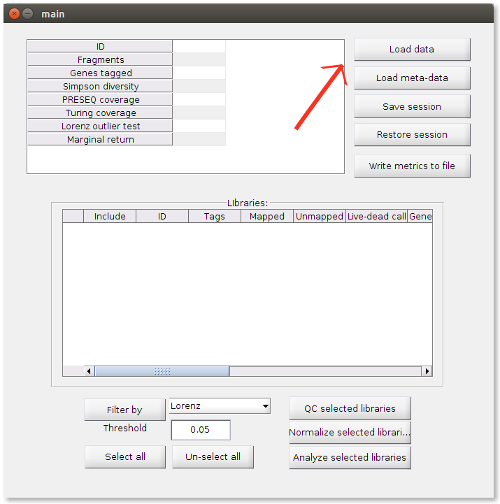
There is also a sample data file included in the source-code , test_data.txt. To import your gene expression dataset into SCell, select Load data in the main window, then choose your raw gene counts file from the dialog box.
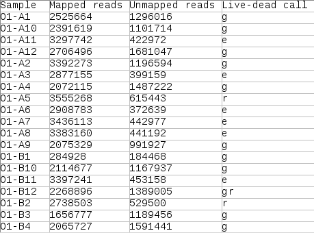
SCell also accepts a metadata table associated with the libraries in your dataset. The metadata table should include:
- a live-dead image call from your single-cell workflow
- number of mapped reads
- number of unmapped reads
The metadata file must have the format shown below.
There is also a sample meta-data file on Github, test_meta_data.txt.To import your metadata into SCell, select Load meta-data in the main window, then choose the corresponding file from the dialog box.
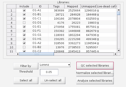
The library names and associated metadata for the imported cells is displayed in the interactive expression profiler in the main window.
SCell can identify low quality libraries by computing their Lorenz statistic. Briefly, it estimates genes expressed at background levels in a given sample, and filters samples whose background fraction is significantly larger than average, via a threshold on the Lorenz statistic's Benjamini-Hochberg corrected q-value.
In our tests, samples that have a small q-value for our Lorenz-statistic have low library complexity, as measured by Gini-Simpson index (Simpson, 1949), and they have low coverage, as estimated by the Good-Turing statistic (Good, 1953). Moreover, in our data the Lorenz-statistic correlates with the results of live-dead staining.
To perform QC on the selected single-cell RNA-seq libraries, select QC selected libraries in the lower panel of the main window.
SCell will estimate library complexity, coverage and the Lorenz statistic for the selected libraries. SCell will prompt you for the location of a PRESEQ executable. If you have PRESEQ installed, SCell will also run it for each of your libraries and estimate the marginal return for resequencing that library from PRESEQ's extrapolation curve. If you don't have PRESEQ installed or don't want to run it just hit cancel when prompted for the PRESEQ location. SCell will then generate the following QC plots:
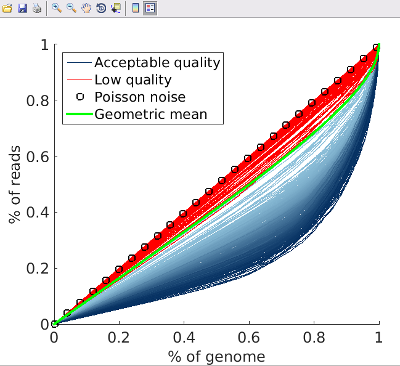
Lorenz Curves
In green, plotted is the cumulative density of the order-statistics (i.e. a sorting) of the reference sample. The reference sample is constructed as the gene-wise geometric means of the individual libraries' read-counts. The cumulative densities of the concomitant-statistics (i.e. re-orderd according to the index that sorts the reference) of the individual libraries are shown in red and blue. That of a low-rate Poisson noise simmulation is shown in black circles. Single-tailed score tests of binomial proportions (with the height of the reference sample as a null hypothesis) are performed at the point where the reference sample maximally diverges from the Poisson noise simulation. Samples whose q-value is less that 0.05 are highlighted in red, all others in blue.
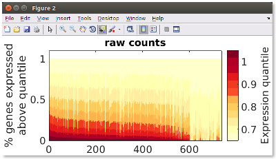
Per-Cell Gene Expression Distribution
This plot provides a summary snapshot of the quality of your data. Each column is a sample, and the percentages of genes expressed above a given expression quantiles are displayed as a stacked bar chart.
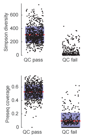
Simpson Diversity and PRESEQ Coverage Boxplots
SCell reports library coverage estimates based on PRESEQ (Daley and Smith, 2014) extrapolation curves, as well as the Simpson diversity statistic.
SCell displays these quality metrics along with the user’s metadata, in the interactive expression profiler.
Once these metrics have been estimated, you may filter low-complexity or outlier cells by selecting Lorenz or PRESEQ from the dropdown menu in the main window lower panel, and setting a threshold to filter by (default=0.05, Lorenz).
Then, click Filter by to unckeck cells that did not meet the established threshold in the interactive expression profiler. This will cause low quality/outlier libraries to be excluded from all downstream analysis.
You may also de-select libraries that you wish to exclude based on other criteria shown in the expression profiler, such as live/dead staining image call or number of genes tagged.
Once your single-cell data has been filtered for low-quality samples, SCell can perform normalization of your libraries in several ways:
a) Normalization by library size (counts per million)
b) Iteratively-reweighted least squares regression (IRLS), with a bi-square weight function, to regress out variation dependent on human cyclin/CDK expression
c) IRLS regression to regress out variation dependent on a user-defined gene list
It is useful to select a discriminating panel of genes for dimensionality reduction (feature selection). An ideal gene for dimensionality reduction is one that is sampled in a large number of cells, while at the same time exhibiting sufficient inter-cellular variance as to distinguish disparate cell types. In the low-coverage regime, typical of single-cell data, it can be difficult to distinguish when a gene is under-sampled due to technical limitations from when it is lowly expressed.
SCell provides statistics for feature selection. It uses a score statistic derived from a generalized-Poisson model, to test for zero-inflation in each gene’s expression across cells. And, SCell uses the index of dispersion (ratio of variance to mean) to estimate a gene's variability, which has a closed form power function.
To normalize samples by library size and select a gene panel for analysis, follow these steps:
-
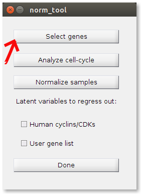
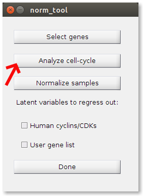
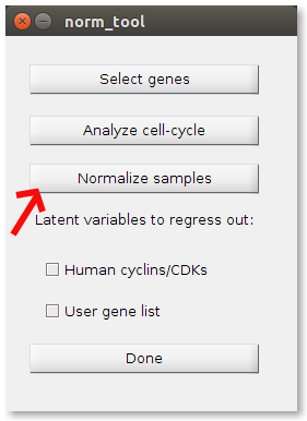
In the main panel, select the Normalize selected libraries button to launch the normalization tool window.
-
Once in the normalization tool, click on Select Genes.
-
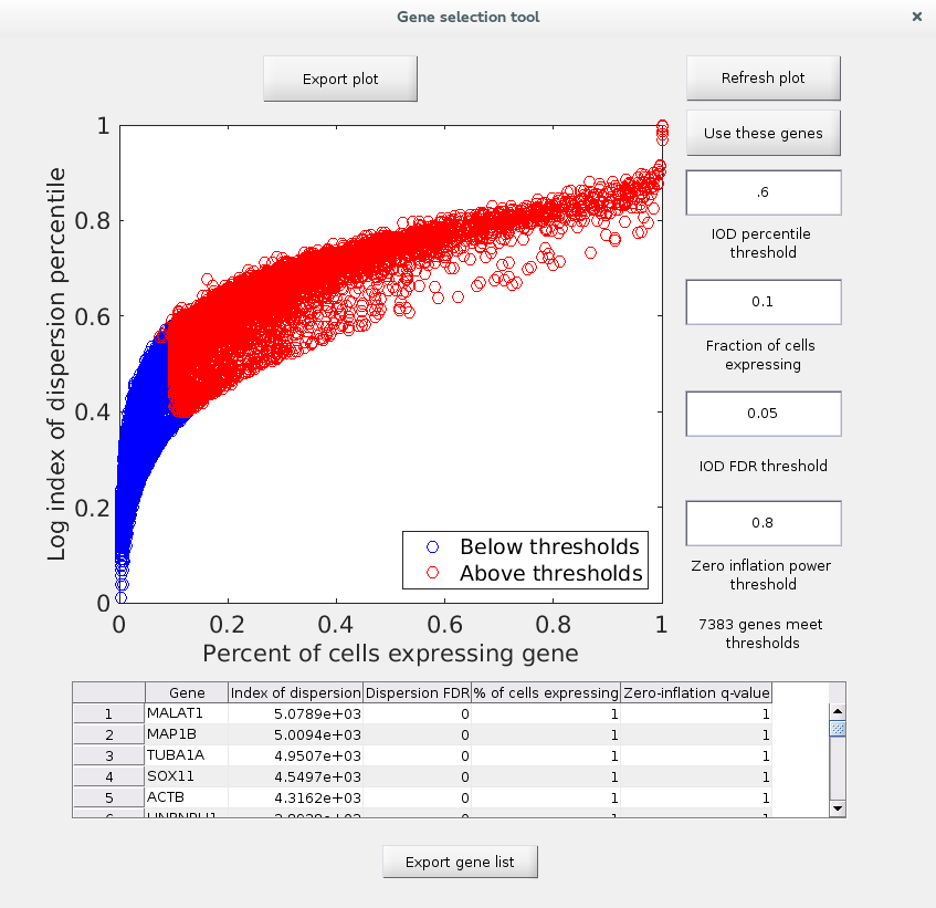
SCell will perform gene variance and zero-inflation analysis, and a Gene Selection Tool window will be launched.
-
In the Gene Selection Tool window, set an Index of Dispersion percentile threshold for genes, as well as a threshold for the fraction of cells expressing a given gene. You can also set a zero-inflation power threshold and a fasle discovery rate threshold on the index of dispersion. On the lower panel, SCell displays a list of the genes in your dataset and their values for these metrics. This list, as well as the displayed plot, can be exported by selecting the Export plot or Export gene list buttons.
-
Once the thresholds for a gene panel have been chosen, click Use these genes. Only the genes that meet your criteria will be used for downstream analysis.
-
You will be taken back to the Normalization Tool window. Click Done.
Your libraries are now normalized by library size (counts per million). You will be taken back to the Main Panel, where you may proceed to dimensionality reduction and clustering of the filtered, normalized libraries.
4b. Assess the correlation of human cyclins and cyclin-dependent kinases with genome-wide expression via cannonical correlation analysis
- Press the Analyze Cell-Cycle button
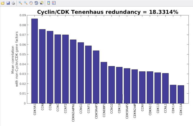
- SCell will estimate the percentage of genome-wide variance explained by cyclin/CDKs, the specific cyclins/CDKs that explain the highest percentage of variance and the genes that correlate most strongly with cyclin/CDKs.
A barchart will be displayed, showing Cyclin/CDK contribution to the observed variance in gene expression.
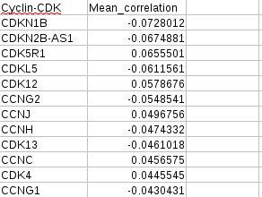
You will be prompted to specify the location to store the file for cyclin/CDK correlations, then for cyclin/CDK-gene correlations. Choose a location in the dialog box, then click Save.
Cyclin-CDK Correlations File
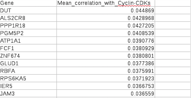
Cyclin-CDK/Gene Correlations File
4c. Normalization by Human Cyclins and Cyclin-Dependent Kinases (Cell Cycle Regression) or a user supplied list
To normalize for the effect of cell cycle on gene expression (remove unwanted variation due to cell cycle state) or to normalize by a user defined set of genes, in addition to normalizing libraries by size, follow these steps:
-
Follow steps 1 to 5 from the Normalization by Library size (CPM) section above, in order to select a meaningful gene panel to include in the analysis.
-
On the Normalization Tool window, check the Human cyclins/CDKs box or the User gene list box, then click Normalize samples.
If you checked User gene list then you will be prompted for a gene list. This should be a text file with one gene name per line, and the gene names must match those used in the original input data file exactly. Normalization may take up to a half-hour to complete. Once the libraries have been normalized, you will be taken back to the Main Panel, where you may proceed to dimensionality reduction and clustering of the filtered, normalized libraries.
SCell can produce counts normalized by any combination of:
-
Cyclins and cyclin-dependent kinases (a model of cell cycle state)
-
A user supplied count matrix (enabling an arbitrary set of controls).
SCell implements PCA for dimensionality reduction, and optionally Varimax-rotation.
On the lower panel of the Main Window, select Analyze selected libraries to perform dimensionality reduction via PCA on the QC-filtered and normalized libraries.
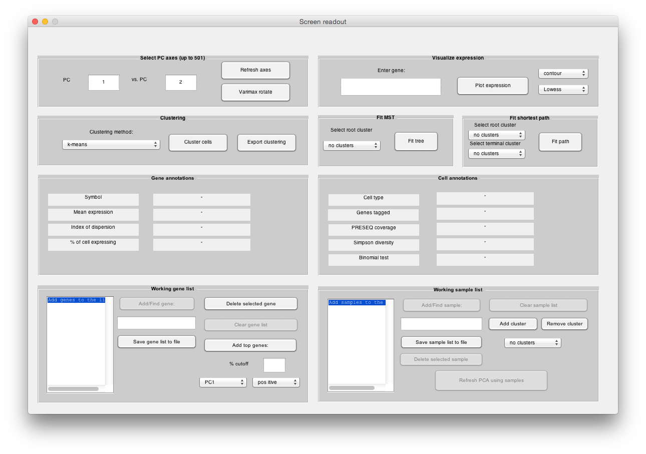
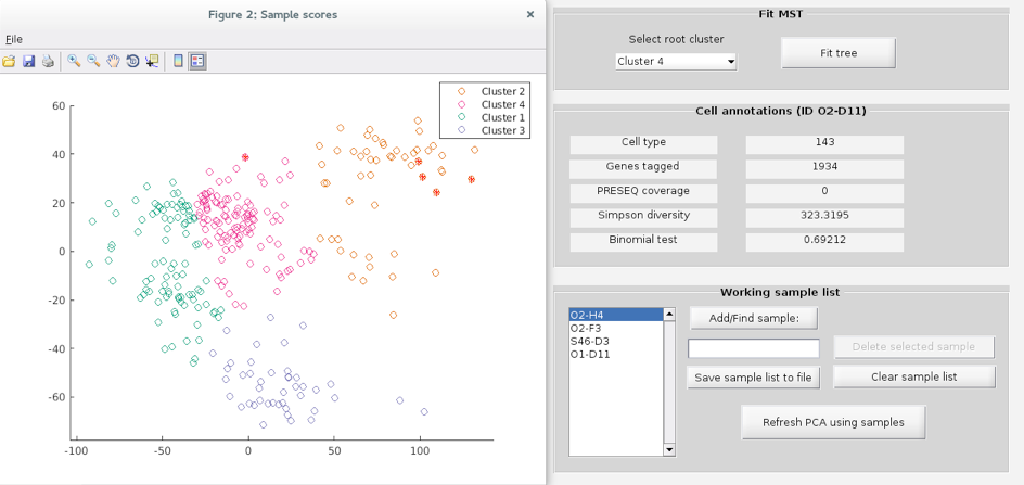
Two interactive plots will be displayed, which allow the user to explore samples in PCA space, with gene-level and sample-level metadata displayed in a third window upon mouse-over:
○ Interactive PCA Sample Scores Plot
View samples in PCA space.
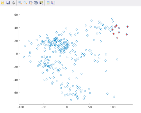
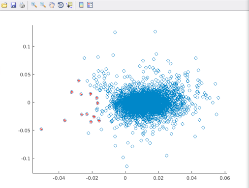
Mouse-over samples to view their identity and associated metrics, or click on a sample to mark and add it to the working sample list. A sample can be removed by pressing escape. By default, PC1 and PC2 are the axes shown on the plot, but this can be modified (see below).
○ Interactive Gene Loadings Plot
In this dataset, canonical neuronal genes load negative PC1.
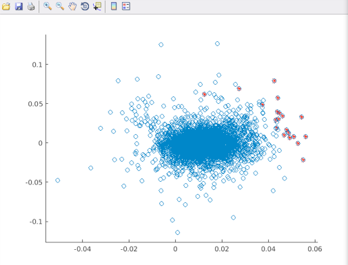
Canonical radial glia (neocortical neural stem cells) marker genes load positive PC1.
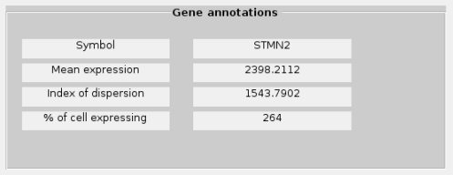
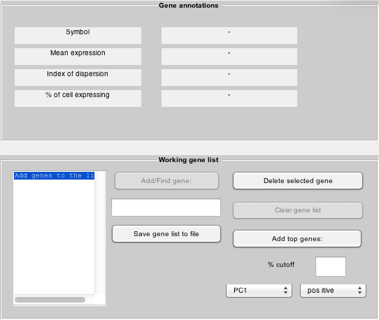
Mouse over genes in the Gene Loading plot to view their gene symbol, mean expression, IOD and the percentage of cells expressing the gene in the Gene Annotations panel.
Click on genes in the gene loading plot to add them to the Working gene list. Alternatively, to find a gene in the loading plot, type its gene symbol in the Working gene list panel search box, then click Add/Find gene. The gene will be highlighted on the loading plot, and added to the working list. Lastly, one can select simultaneously (and add to the working gene list) the top loading genes of a given PCA direction based on a threshold.
The current working gene list can be exported to a file for downstream analysis, by selecting Save gene list to file in the Working gene list panel. You will be prompted to choose a location to store the file.
By default, PC1 and PC2 are the axes shown on the PCA score and loading plots, but this can be modified. Enter the axes you would like to plot, then select Refresh PCA axes to generate new Sample Scores and Gene Loadings plots.
You can apply Varimax Rotation to post-process the PCA, a technique which will decrease the number of genes that load both PCA axes to a comparable degree and can make the PCA axes more interpretable. To apply Varimax rotation, simply click Varimax rotate. The plots will be updated accordingly.
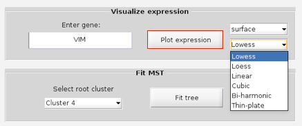
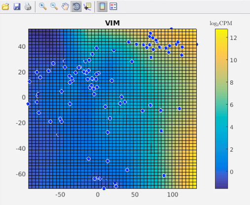
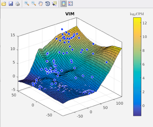
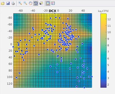
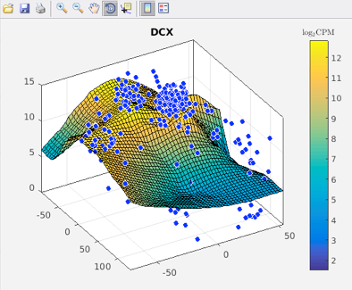
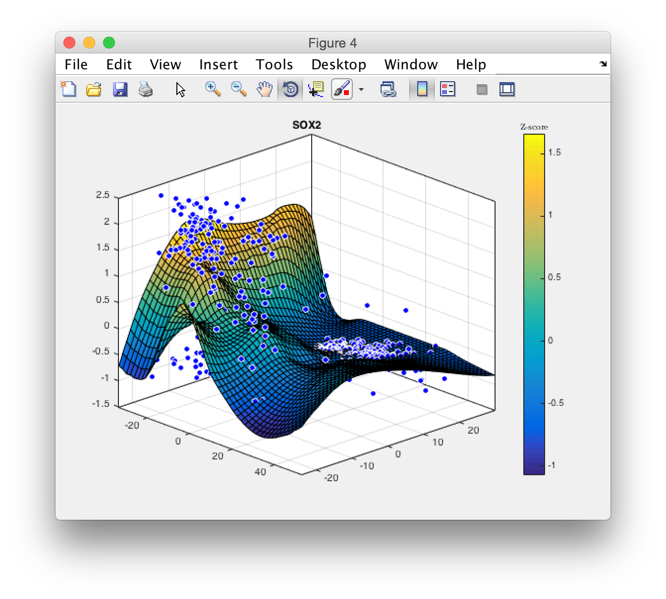
SCell can be used to visualize gene expression as a regression or interpolation across PCA coordinates. To visualize a gene of interest, enter the name and select surface or contour. Select a regression method from the drop-down menu, then click on Plot expression to generate a plot of gene expression across cells in PCA space.
For example, we plot the expression of VIM and DCX, a radial glia and newborn neuron marker respectively.
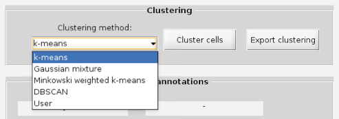
SCell implements 4 different clustering algorithms:
○ k-means
○ Gaussian mixture
○ Minkowski weighted k-means
○ DBSCAN
In the Clustering panel, select one of the clustering algorithms from the drop-down menu, then click Cluster cells.
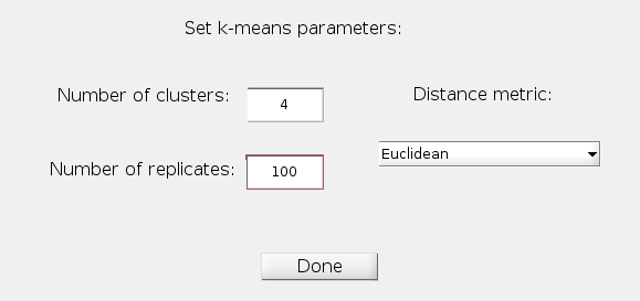
A new window will prompt you to enter the desired number of clusters, as well as the number of replicates and distance metric to use. Enter these parameters, then click Done.
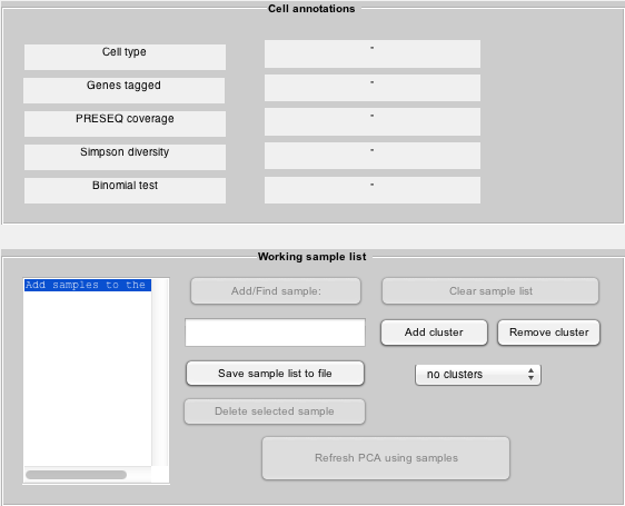
The sample-score window will now be color-coded according to their assigned cluster. In addition to adding samples to the Working sample list by clicking individual samples, you can now add all samples in a cluster at once. This could for example be used to run a new PCA to subcluster a given cluster.
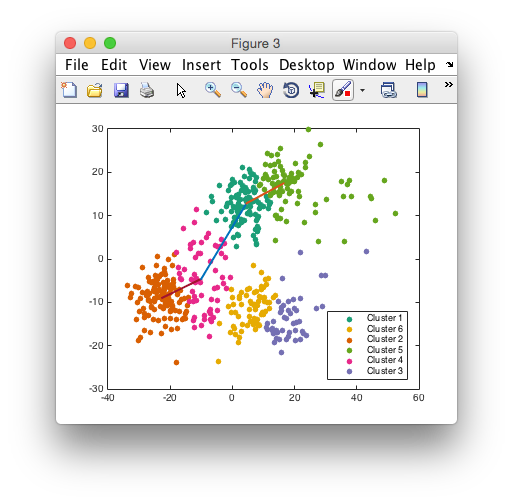
Once cells have been clustered, SCell can compute a Minimum Spanning Tree or a Gabriel graph minimum cost path, to predict a lineage trajectory across clusters. Select a root cluster from the drop-down menu in the Fit MST panel, then click Fit Tree, or select the root cluster and terminal cluster and click Fit path.
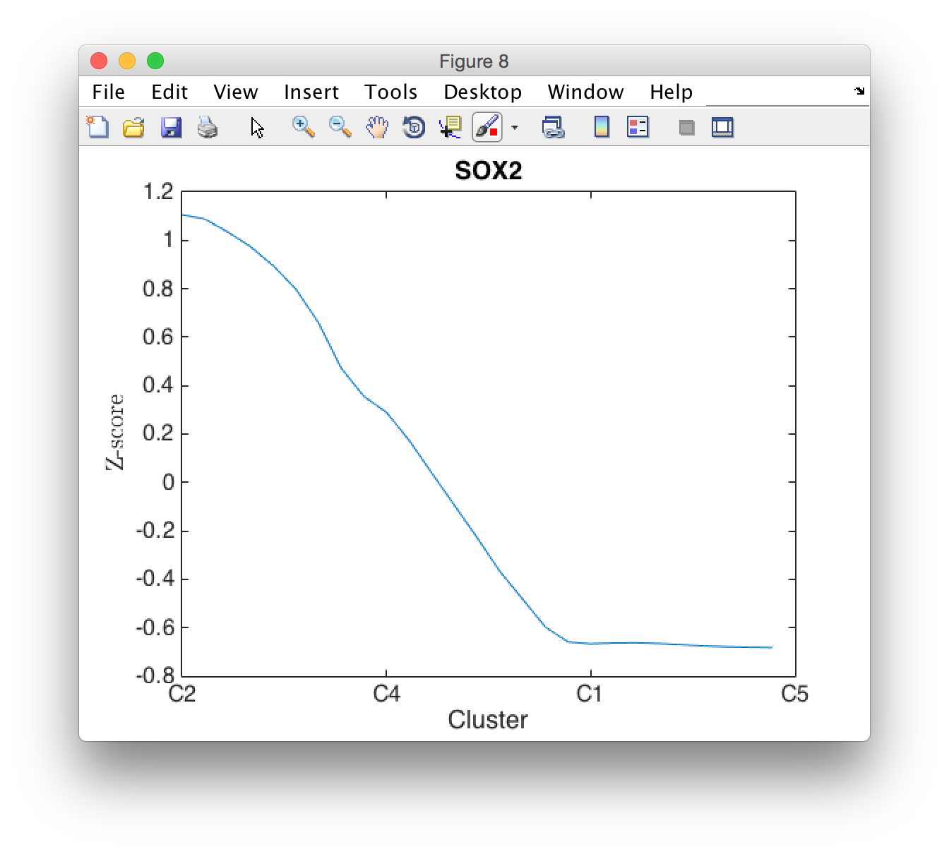
A shortest-path or a MST will then be fit. All subsequent gene visualizations (i.e. clicking the Plot expression button) will then produce expression estimates along this path or tree, and a new plot will be generated with the path or tree highlighted.
SCell can perform PCA on a subset of libraries selected from the first round of analysis. Select cells individualy or select an entire clsuter at once using the Add cluster button and dropdown.

The selected samples will appear on the Working Sample List in the main panel and be highlighted in the scatter-plot. Click Refresh PCA using samples to perform a new iteration of PCA on the selected libraries only. A new sample scores plot will be displayed containing only the selected libraries in PCA space. You can choose to apply Varimax rotation as described above, or to change the principal components plotted on each axis. A new gene loading plot will be displayed as well, showing the new contribution of genes to each principal component shown. The expression of selected genes across this subset of samples can be displayed as described above. Samples can be clustered and a new minimum-spanning tree can be fit to further characterize the subset of cells being analyzed.
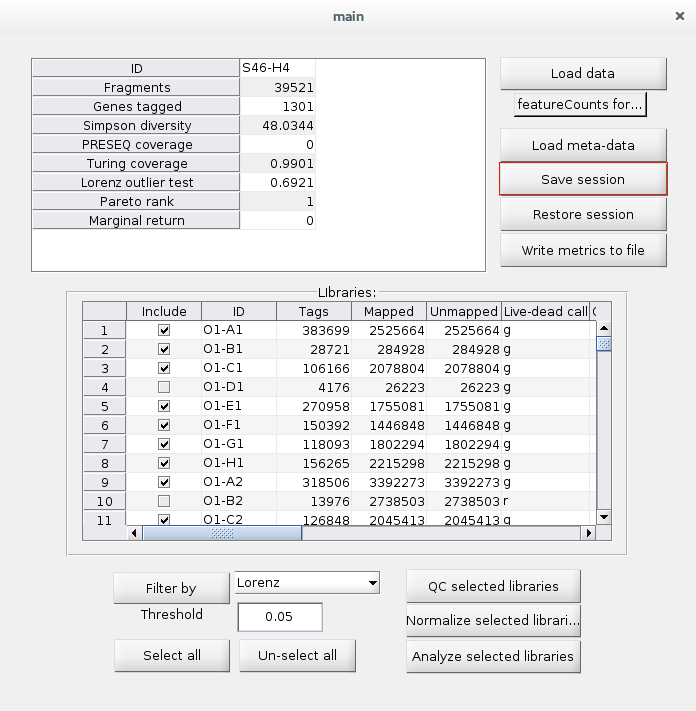
To save the current session, including library QC and filtering, feature selection and normalization, select Save Session on the main window.
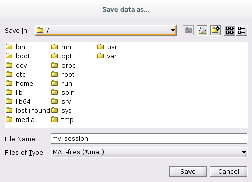
You will be prompted to choose a location to store the .mat session. Choose a name for the session, and click Save.
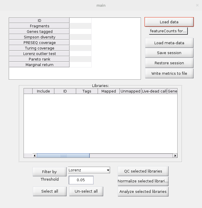
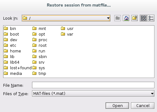
To restore a previously saved session into SCell, select Load data on the main window.
You will be prompted to select the .mat file you wish to load. Once the file has been selected, select Open. Your data, selected libraries, feature selection and normalization, will be restored.
In the folder preproc_scripts you can find scripts to trim, align and perform read-level QC on large ensembles of single-cell RNA-seq libraries. These scripts are written to be run on a high-performance computing cluster running the Torque resource manager. All of them have the property that they take as input a directory containing sub-directories in which are stored the files corresponding to individual libraries for individual cells. The assumed arangement of raw data is a folder corresponding to a sample or sequencing run, with one sub-folder per single-cell library. Each sub-folder should then contain the raw reads as compressed FASTQ files. The scripts assume that you have paired-end reads. You will need to edit these scripts to match your read type. Jobs that process individual libraries are instantiated in an array. The number of jobs run concurrently, the number of threads to use and which references to use in the alignment and gene quantification can be set as parameters. These scripts are provided "as is" in an effort to be useful and save you some typing, they are not gauranteed to be suitable for any particular purpose.
We use TrimGalore!, which employs cutadapt to trim adapter sequences, as well as to trim low quality bases at the ends of reads.
To trim reads, run the shell script sub_trim.sh from the terminal, specifying the directory of single-cell libraries you want to trim. This usually corresponds to a sequencing plate of single-cell libraries.
sh sub_trim.sh sequencingRunDirThis script calls and executes the PBS script trim.pbs. A new subdirectory called /trimmed will be created under each individual library's directory, which now contains the quality-and-barcode-trimmed reads in a fastq file. The /trimmed subdirectory will also contain the output from FastQC for each individual library in your sequencing run. This will allow you to inspect read-level quality metrics. A MATLAB script to summarize read-level QC by sequencing run is also provided: summarize_fastqc.m.
The scripts provided here make use of TopHat 2, a splice junction short read aligner for RNA-Seq data. To align your single-cell libraries, run the shell script sub_align.sh from the terminal, specifying the directory of single-cell libraries you wish to align. This script calls and executes the PBS script align.pbs, which will submit the alignment jobs for each of the trimmed libraries in the specified directory as a job array.
sh sub_align.sh /path/to/sequencingRunDirIn the sub_align.sh script, you must specify:
• The path to the Bowtie genome index directory containing the necessary .bt2 files for alignment.
• The path to the transcriptome index containing the necessary .bt2 files to be used for the guided alignment.
• The base name for the .bt2 files in the Bowtie genome index directory to be used for alignment.
This script will create a new directory called /tophat_out, which contains one sub-directory per library. In each sub-directory is placed the .bam files and other Tophat2 output, as well as alignment summary statistics corresponding to each single-cell library. Mapping rate statistics contained in the file accepted_hits.stats from each library can be summarized by running the script comp_mapping_rates.m.
FeatureCounts, part of the SubRead package, assigns aligned reads/fragments to genomic features, such as genes.
The output of this read summarization process is a counts matrix, which contains the number of reads/fragments assigned to each feature for each one of your single-cell libraries. To obtain a matrix of gene counts from your aligned single-cell libraries, run the shell script sub_featureCounts.sh from the terminal, specifying the name of the single-cell library directory to summarize.
sh sub_featureCounts.sh sequencingRunDirThis script calls the PBS script run_featureCounts.pbs. You will need a GTF file containing the features you want to summarize aligned reads to. In the run_featureCounts.pbs file, you must specify the path to the GTF file to use for read summarization. This will create a new directory named /featureCounts_out, which contains a tab-delimited text file with genes as rows, and columns as single-cell libraries. This matrix is ready to be imported into SCell for quality control and analysis, but you must remove columns 2-6 and remove the first header line, for example cut -f1,7-${num_of_libs} my_counts.txt >final_counts.txt to remove columns 2-6 and delete the first headerline in a text editor.
