Exercises for Laboratory of Computational Physics mod. A

Physics of Data @ University of Padova - October 2022 ~ January 2023

Exercises that are intended to show that I know Python and standard data analysis techniques.

Diffusion using random walk

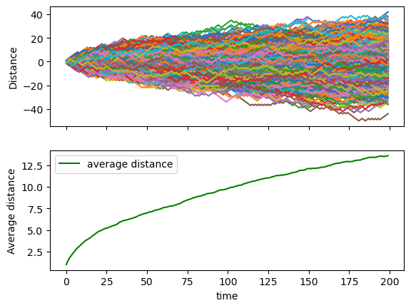
Consider a simple random walk process: at each step in time, a walker jumps right or left (+1 or -1) with equal probability. The goal is to find the typical distance from the origin of a random walker after a given amount of time. To do that, let's simulate many walkers and create a 2D array with each walker as a row and the actual time evolution as columns

Take 1000 walkers and let them walk for 200 steps
Use randint to create a 2D array of size walkers x steps with values -1 or 1
Build the actual walking distances for each walker (i.e. another 2D array "summing on each row")
Take the square of that 2D array (elementwise)
Compute the mean of the squared distances at each step (i.e. the mean along the columns)
Plot the average distances (sqrt(distance**2)) as a function of time (step)

Did you get what you expected?

Kernel Density Estimate

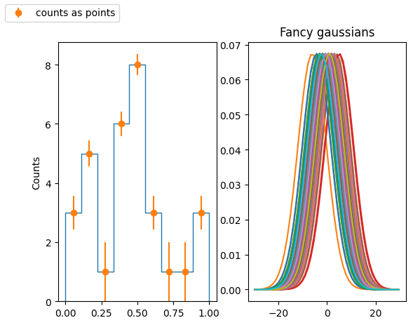
Produce a KDE for a given distribution (by hand, not using seaborn!):

Fill a numpy array, x, of len(N) (with N=O(100)) with a variable normally distributed, with a given mean a standard deviation
Fill an histogram in pyplot taking properly care about the aesthetic
- use a meaningful number of bins
- set a proper y axis label
- set proper value of y axis major ticks labels (e.g. you want to display only integer labels)
- display the histograms as data points with errors (the error being the poisson uncertainty)
for every element of x, create a gaussian with the mean corresponding the element value and std as a parameter that can be tuned. The std default value should be: $$ 1.06 * x.std() * x.size ^{-\frac{1}{5.}} $$ you can use the scipy function stats.norm() for that.
In a separate plot (to be placed beside the original histogram), plot all the gaussian functions so obtained
Sum (with np.sum()) all the gaussian functions and normalize the result such that the integral matches the integral of the original histogram. For that you could use the scipy.integrate.trapz() method

Linear algebra - PCA on 3D dataset

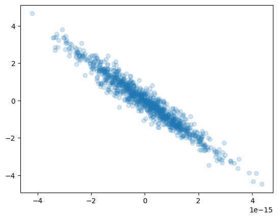
Generate a dataset with 3 features each with N entries (N being ${\cal O}(1000)$). With $N(\mu,\sigma)$ the normal distribution with mean $\mu$ and $\sigma$ standard deviation, generate the 3 variables $x_{1,2,3}$ such that:
- $x_1$ is distributed as $N(0,1)$
- $x_2$ is distributed as $x_1+N(0,3)$
- $x_3$ is given by $2x_1+x_2$
Find the eigenvectors and eigenvalues of the covariance matrix of the dataset
Find the eigenvectors and eigenvalues using SVD. Check that the two procedures yield to same result
What percent of the total dataset's variability is explained by the principal components? Given how the dataset was constructed, do these make sense? Reduce the dimensionality of the system so that at least 99% of the total variability is retained.
Redefine the data in the basis yielded by the PCA procedure
Plot the data points in the original and the new coordiantes as a set of scatter plots. Your final figure should have 2 rows of 3 plots each, where the columns show the (0,1), (0,2) and (1,2) proejctions.

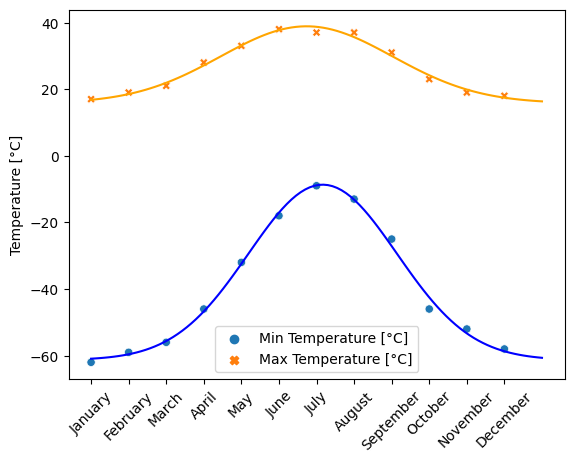
Cruve fitting of temperature in Alaska

The temperature extremes in Alaska for each month, starting in January, are given by (in degrees Celcius):

max: 17, 19, 21, 28, 33, 38, 37, 37, 31, 23, 19, 18

min: -62, -59, -56, -46, -32, -18, -9, -13, -25, -46, -52, -58

Plot these temperature extremes.
Define a function that can describe min and max temperatures.
Fit this function to the data with scipy.optimize.curve_fit().
Plot the result. Is the fit reasonable? If not, why?
Is the time offset for min and max temperatures the same within the fit accuracy?

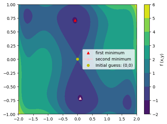
2D minimization of a six-hump camelback function**

$$ f(x,y) = \left(4-2.1x^2+\frac{x^4}{3} \right) x^2 +xy + (4y^2 -4)y^2 $$

has multiple global and local minima. Find the global minima of this function.

Hints:

Variables can be restricted to $-2 < x < 2$ and $-1 < y < 1$.
Use numpy.meshgrid() and pylab.imshow() to find visually the regions.
Use scipy.optimize.minimize(), optionally trying out several of its methods.

How many global minima are there, and what is the function value at those points? What happens for an initial guess of $(x, y) = (0, 0)$ ?

Montecarlo - Radioactive decay chain

${\rm Tl}^{208}$ decays to ${\rm Pb}^{208}$ with a half-life of 3.052 minutes. Suppose to start with a sample of 1000 Thallium atoms and 0 of Lead atoms.

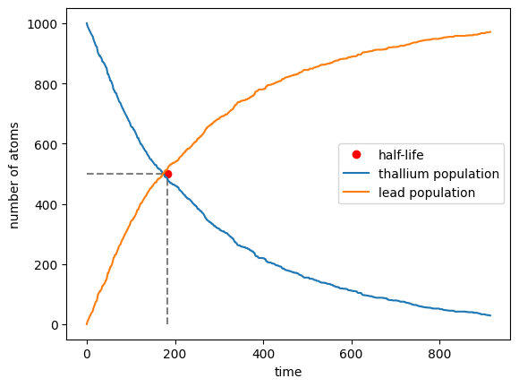
Take steps in time of 1 second and at each time-step decide whether each Tl atom has decayed or not, accordingly to the probability $p(t)=1-2^{-t/\tau}$. Subtract the total number of Tl atoms that decayed at each step from the Tl sample and add them to the Lead one. Plot the evolution of the two sets as a function of time
Repeat the exercise by means of the inverse transform method: draw 1000 random numbers from the non-uniform probability distribution $p(t)=2^{-t/\tau}\frac{\ln 2}{\tau}$ to represent the times of decay of the 1000 Tl atoms. Make a plot showing the number of atoms that have not decayed as a function of time

diegobonato/LaboratoryOfComputationalPhysicsModA