HPBdata

HPBdata aims to provide access to historical meteorological measurements at various temporal resolutions (1 min, 10 min, 1 day) obtained at ‘Hohenpeißenberg’ site (Bavaria, Germany). Data was acquired from the Climate Data Center hosted by the German Weather Service and has been coverted to {xts} objects for subsequent applications in need of representative meteorological measurements.

Since I found myself in the need of a meteorological measurement sample dataset for climatological evaluations, meteorological calculations, extreme value statistics, etc quite often, I decided to assemble needed data in order to simplify package development in the future.

Installation

You can install the development version of HPBdata with:

# install.packages("devtools")
devtools::install_github("dimfalk/HPBdata")

and load the package via

library(HPBdata)
#> 0.1.6

Getting started

There is not really much to say about the use. HPBdata is a data-only package without any functions provided consisting of three objects:

obs_1min, obs_10min and obs_1d.

These are named lists of different length containing xts objects of different length at specified interval width for various meteorological parameters.

For details, it is strongly encouraged to study the dataset documentation provided, e.g. ?obs_10min, and the official dataset description linked there.

# inspect superordinate list
class(obs_10min)
#> [1] "list"

length(obs_10min)
#> [1] 9

names(obs_10min)
#> [1] "PP_10"  "TT_10"  "TM5_10" "RF_10"  "FF_10"  "DD_10"  "GS_10"  "SD_10" 
#> [9] "RWS_10"

# inspect xts objects contained
class(obs_10min[["TT_10"]])
#> [1] "xts" "zoo"

length(obs_10min[["TT_10"]])
#> [1] 1581036

As a little remark worth noting, the xts objects contained are provided with some additional metadata appended in form of attributes based on a data model implemented in {timeseriesIO} to ensure I/O compatibility:

attributes(obs_10min[["TT_10"]])[5:22]
#> $MEAS_RESOLUTION
#> [1] 10
#> 
#> $STAT_ID
#> [1] "02290"
#> 
#> $STAT_NAME
#> [1] "Hohenpeißenberg"
#> 
#> $X
#> [1] 11.0108
#> 
#> $Y
#> [1] 47.8009
#> 
#> $Z
#> [1] 977
#> 
#> $CRS_EPSG
#> [1] "4326"
#> 
#> $HRS_EPSG
#> [1] NA
#> 
#> $TZONE
#> [1] "UTC"
#> 
#> $PARAMETER
#> [1] "Lufttemperatur"
#> 
#> $TS_START
#> [1] "1993-12-09 13:50:00 UTC"
#> 
#> $TS_END
#> [1] "2023-12-31 23:40:00 UTC"
#> 
#> $TS_DEFLATE
#> [1] FALSE
#> 
#> $TS_TYPE
#> [1] "measurement"
#> 
#> $MEAS_INTERVALTYPE
#> [1] TRUE
#> 
#> $MEAS_BLOCKING
#> [1] "left"
#> 
#> $MEAS_UNIT
#> [1] "°C"
#> 
#> $MEAS_STATEMENT
#> [1] "mean"

Other than that, you can now just leverage all the sweet xts functionality:

library(xts)
#> Lade nötiges Paket: zoo
#> 
#> Attache Paket: 'zoo'
#> Die folgenden Objekte sind maskiert von 'package:base':
#> 
#>     as.Date, as.Date.numeric

# subsetting
x <- obs_10min[["TT_10"]]["2022"]
x
#>                     TT_10
#> 2022-01-01 00:00:00   9.2
#> 2022-01-01 00:10:00   9.2
#> 2022-01-01 00:20:00   9.1
#> 2022-01-01 00:30:00   9.0
#> 2022-01-01 00:40:00   8.8
#> 2022-01-01 00:50:00   8.7
#> 2022-01-01 01:00:00   8.6
#> 2022-01-01 01:10:00   8.5
#> 2022-01-01 01:20:00   8.5
#> 2022-01-01 01:30:00   8.3
#>                 ...      
#> 2022-12-31 22:20:00  12.2
#> 2022-12-31 22:30:00  13.0
#> 2022-12-31 22:40:00  12.9
#> 2022-12-31 22:50:00  13.4
#> 2022-12-31 23:00:00  14.2
#> 2022-12-31 23:10:00  15.3
#> 2022-12-31 23:20:00  14.9
#> 2022-12-31 23:30:00  14.7
#> 2022-12-31 23:40:00  14.1
#> 2022-12-31 23:50:00  11.4

# aggregating
xts::apply.monthly(x, "mean", na.rm = TRUE) |> round(1)
#>                     TT_10
#> 2022-01-31 23:50:00   0.5
#> 2022-02-28 23:50:00   1.8
#> 2022-03-31 23:50:00   4.8
#> 2022-04-30 23:50:00   5.7
#> 2022-05-31 23:50:00  13.2
#> 2022-06-30 23:50:00  17.2
#> 2022-07-31 23:50:00  18.2
#> 2022-08-31 23:50:00  17.8
#> 2022-09-30 23:50:00  11.4
#> 2022-10-31 23:50:00  13.4
#> 2022-11-30 23:50:00   5.9
#> 2022-12-31 23:50:00   1.3

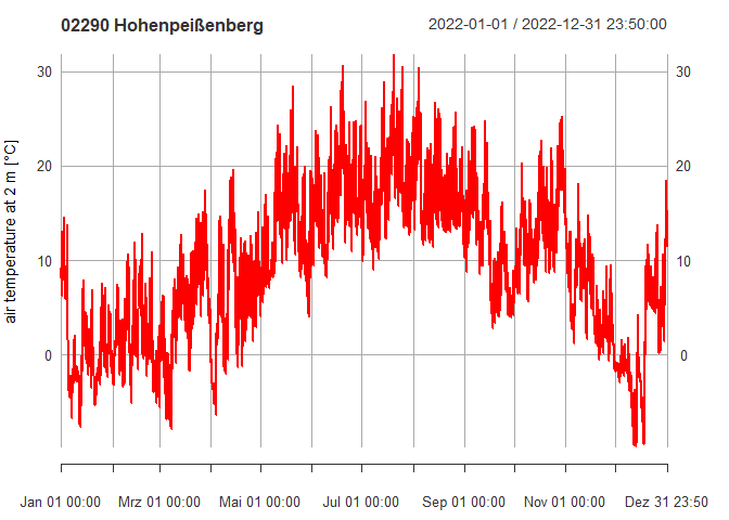
# plotting
plot(x, ylab = "air temperature at 2 m [°C]", col = "red", main = "02290 Hohenpeißenberg")