- Load the ‘divorce_margarine’ dataset from the ‘dslabs’ package.
dataset.divorce_margarine <- dslabs::divorce_margarine
dataset.divorce_margarine
## # A tibble: 10 × 3
## divorce_rate_maine margarine_consumption_per_capita year
## <dbl> <dbl> <int>
## 1 5 8.2 2000
## 2 4.7 7 2001
## 3 4.6 6.5 2002
## 4 4.4 5.3 2003
## 5 4.3 5.2 2004
## 6 4.1 4 2005
## 7 4.2 4.6 2006
## 8 4.2 4.5 2007
## 9 4.2 4.2 2008
## 10 4.1 3.7 2009
- Investigate the correlation between margarine consumption and divorce rates in Maine.
ggplot(dataset.divorce_margarine, aes(x = margarine_consumption_per_capita, y = divorce_rate_maine)) +
  geom_point(size = 3) +
  geom_smooth(method = "lm", formula = y ~ x, color = COLORS[5], fill = COLORS[4]) +
  labs(
    x = "Margarine Consumption per Capita",
    y = "Divorce Rate in Maine",
  )
lm(
data = dataset.divorce_margarine,
formula = divorce_rate_maine ~ margarine_consumption_per_capita,
) %>% summary()##
## Call:
## lm(formula = divorce_rate_maine ~ margarine_consumption_per_capita,
## data = dataset.divorce_margarine)
##
## Residuals:
## Min 1Q Median 3Q Max
## -0.0558 -0.0182 -0.0145 0.0360 0.0462
##
## Coefficients:
## Estimate Std. Error t value Pr(>|t|)
## (Intercept) 3.30863 0.04803 68.9 2.2e-12 ***
## margarine_consumption_per_capita 0.20139 0.00874 23.1 1.3e-08 ***
## ---
## Signif. codes: 0 '***' 0.001 '**' 0.01 '*' 0.05 '.' 0.1 ' ' 1
##
## Residual standard error: 0.0384 on 8 degrees of freedom
## Multiple R-squared: 0.985, Adjusted R-squared: 0.983
## F-statistic: 532 on 1 and 8 DF, p-value: 1.33e-08
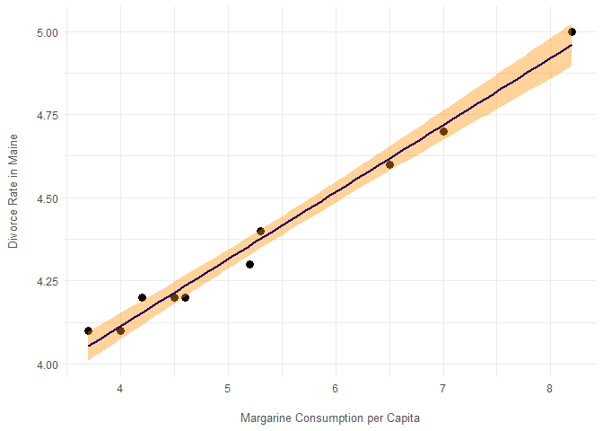
Modelling the divorce rate in Maine as a linear function of margarine consumption per capita yields a R2-coefficient of 0.985, seemingly indicating that more than 98% of the variation in divorce rates is accounted for by variation in margarine consumption.
- Would an increase in the preference for margarine lead to skyrocketing divorce rates?
Trusting the model naïvely would lead to the implication that increased margarine consumption would cause an increase in divorce rates in Maine. However, it seems much more likely that this is a case of spurious correlation, where a statistical relationship has arisen from random natural variations, such that margarine consumption does not, in fact, have any (direct) influence on divorce rates in Maine.
- Load the ‘GSSvocab’ dataset from the ‘car’ package. This dataset contains people’s scores on an English vocabulary test and includes demographic information.
dataset.car <- carData::GSSvocab
dataset.car
## # A tibble: 28,867 × 8
## year gender nativeBorn ageGroup educGroup vocab age educ
## <fct> <fct> <fct> <fct> <fct> <dbl> <dbl> <dbl>
## 1 1978 female yes 50-59 12 yrs 10 52 12
## 2 1978 female yes 60+ <12 yrs 6 74 9
## 3 1978 male yes 30-39 <12 yrs 4 35 10
## 4 1978 female yes 50-59 12 yrs 9 50 12
## 5 1978 female yes 40-49 12 yrs 6 41 12
## 6 1978 male yes 18-29 12 yrs 6 19 12
## 7 1978 male yes 18-29 12 yrs 4 19 12
## 8 1978 male yes 50-59 12 yrs 7 59 12
## 9 1978 female yes 40-49 16 yrs 8 49 16
## 10 1978 male yes 18-29 12 yrs 3 21 12
## # ℹ 28,857 more rows
- Filter for the year 1978 and remove rows with missing values (the function na.exclude() is one way to do this – check out the documentation!).
dataset.car.1978 <- dataset.car %>%
  subset(year == 1978) %>%
  drop_na()
dataset.car.1978
## # A tibble: 1,477 × 8
## year gender nativeBorn ageGroup educGroup vocab age educ
## <fct> <fct> <fct> <fct> <fct> <dbl> <dbl> <dbl>
## 1 1978 female yes 50-59 12 yrs 10 52 12
## 2 1978 female yes 60+ <12 yrs 6 74 9
## 3 1978 male yes 30-39 <12 yrs 4 35 10
## 4 1978 female yes 50-59 12 yrs 9 50 12
## 5 1978 female yes 40-49 12 yrs 6 41 12
## 6 1978 male yes 18-29 12 yrs 6 19 12
## 7 1978 male yes 18-29 12 yrs 4 19 12
## 8 1978 male yes 50-59 12 yrs 7 59 12
## 9 1978 female yes 40-49 16 yrs 8 49 16
## 10 1978 male yes 18-29 12 yrs 3 21 12
## # ℹ 1,467 more rows
- Is a person’s score on the vocabulary test (‘vocab’) significantly impacted by their level of education (‘educ’)? Visualize the relationship in a plot and build a model. Briefly explain the results.
ggplot() +
  geom_point(
    data = dataset.car.1978,
    aes(x = educ, y = vocab),
    size = 2,
    alpha = 0.2,
    position = position_jitter(width = 0.4, height = 0.2),
  ) +
  geom_smooth(
    data = dataset.car.1978,
    aes(x = educ, y = vocab),
    method = "lm",
    formula = y ~ x,
    color = COLORS[5],
    fill = COLORS[4],
  ) +
  scale_x_continuous(breaks = seq(0, 20)) +
  scale_y_continuous(breaks = seq(0, 10)) +
  labs(
    x = "Years of Education",
    y = "Vocabulary Test Score",
  )
lm(
data = dataset.car.1978,
formula = vocab ~ educ,
) %>% summary()##
## Call:
## lm(formula = vocab ~ educ, data = dataset.car.1978)
##
## Residuals:
## Min 1Q Median 3Q Max
## -7.123 -1.161 0.054 1.092 5.624
##
## Coefficients:
## Estimate Std. Error t value Pr(>|t|)
## (Intercept) 1.2357 0.1996 6.19 7.7e-10 ***
## educ 0.3925 0.0161 24.44 < 2e-16 ***
## ---
## Signif. codes: 0 '***' 0.001 '**' 0.01 '*' 0.05 '.' 0.1 ' ' 1
##
## Residual standard error: 1.89 on 1475 degrees of freedom
## Multiple R-squared: 0.288, Adjusted R-squared: 0.288
## F-statistic: 597 on 1 and 1475 DF, p-value: <2e-16
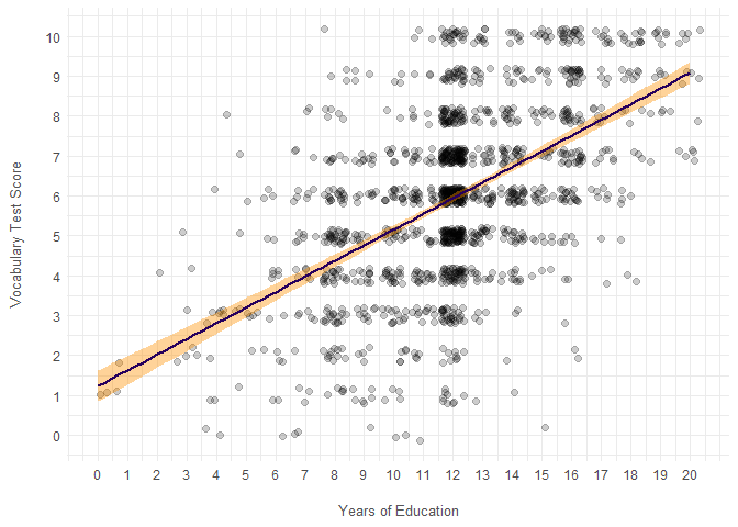
Modelling the vocabulary test score as a linear function of level of education indicates that for each additional year of education, we would, all else being equal, predict an increase in vocabulary test score of 0.39, while an individual with 0 education is predicted to score 1.84 on the vocabulary test. However, the relationship is somewhat diffuse with a modest 29% of co-variation being explained by the model.
- Whether a person is the native of an English-speaking country (‘nativeBorn’) could potentially have an impact on the size of their vocabulary. Visualize the relationship and add the predictor to the model. Briefly explain the results.
ggplot(dataset.car.1978) +
  stat_histinterval(aes(vocab, y = nativeBorn, fill = nativeBorn), alpha = 0.6, na.rm = TRUE, breaks = seq(0, 11), align = 0.5) +
  scale_fill_manual(breaks = c("no", "yes"), labels =  c("Native", "Second Language"), values = COLORS[5:4]) +
  scale_y_discrete(labels = c("Second Language", "Native")) +
  coord_cartesian(ylim = c(1.5, 2)) +
  scale_x_continuous(breaks = seq(0, 10)) +
  guides(fill="none") +
  labs(
    x = "Vocabulary Test Score",
    y = "",
  )
lm(
data = dataset.car.1978,
formula = vocab ~ educ + nativeBorn,
) %>% summary()##
## Call:
## lm(formula = vocab ~ educ + nativeBorn, data = dataset.car.1978)
##
## Residuals:
## Min 1Q Median 3Q Max
## -7.162 -1.201 0.015 1.231 5.803
##
## Coefficients:
## Estimate Std. Error t value Pr(>|t|)
## (Intercept) 0.628 0.277 2.27 0.0233 *
## educ 0.392 0.016 24.50 <2e-16 ***
## nativeBornyes 0.650 0.205 3.16 0.0016 **
## ---
## Signif. codes: 0 '***' 0.001 '**' 0.01 '*' 0.05 '.' 0.1 ' ' 1
##
## Residual standard error: 1.88 on 1474 degrees of freedom
## Multiple R-squared: 0.293, Adjusted R-squared: 0.292
## F-statistic: 306 on 2 and 1474 DF, p-value: <2e-16
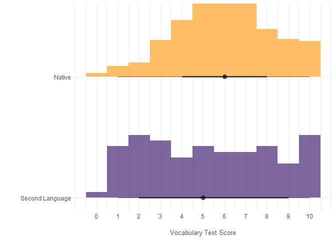
It seems that, on average, native speakers score slightly higher on the vocabulary test but vocabulary scores are more uniformly distributed for non-natives, such that the non-natives are more likely to score either very lowly or very highly.
The linear model would suggest that being a native increases the predicted vocabulary test score by 0.65, although this didn’t really notably increase the proportion of variance explained.
- Does a person’s level of education depend on whether they are a native of the country? Visualize the relationship.
ggplot(dataset.car.1978) +
  stat_histinterval(aes(educ, y = nativeBorn, fill = nativeBorn), alpha = 0.6, na.rm = TRUE, breaks = seq(0, 21), align = 0.5) +
  scale_fill_manual(breaks = c("no", "yes"), labels =  c("Native", "Second Language"), values = COLORS[5:4]) +
  scale_y_discrete(labels = c("Second Language", "Native")) +
  coord_cartesian(ylim = c(1.5, 2)) +
  scale_x_continuous(breaks = seq(0, 20)) +
  guides(fill="none") +
  labs(
    x = "Years of Education",
    y = "",
)- Do you think it makes sense to add the relationship as an interaction term? Try creating the model and briefly explain the results.
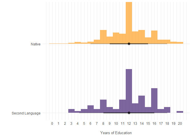
The level of education does not seem to depend on whether one is a native or not. The distributions of education levels don’t differ in any meaningful way.
lm(
  data = dataset.car.1978,
  formula = vocab ~ educ * nativeBorn,
) %>% summary()
##
## Call:
## lm(formula = vocab ~ educ * nativeBorn, data = dataset.car.1978)
##
## Residuals:
## Min 1Q Median 3Q Max
## -7.155 -1.205 0.015 1.235 5.986
##
## Coefficients:
## Estimate Std. Error t value Pr(>|t|)
## (Intercept) 0.3539 0.6878 0.51 0.61
## educ 0.4151 0.0550 7.55 7.4e-14 ***
## nativeBornyes 0.9500 0.7186 1.32 0.19
## educ:nativeBornyes -0.0250 0.0575 -0.44 0.66
## ---
## Signif. codes: 0 '***' 0.001 '**' 0.01 '*' 0.05 '.' 0.1 ' ' 1
##
## Residual standard error: 1.88 on 1473 degrees of freedom
## Multiple R-squared: 0.293, Adjusted R-squared: 0.292
## F-statistic: 204 on 3 and 1473 DF, p-value: <2e-16
By adding an interaction term between nativeness and education, the model finds that, if anything, the effect of education on vocabulary score seems to be marginally smaller for natives, although the parameter estimate is highly uncertain and does not rule out the opposite scenario, i.e. that the effect is in fact larger for natives.
- Which model performs best?
While adding nativeness and its interaction with education did marginally improve the proportion of variance explained, the interaction term did not allow for better prediction. Thus, the model using years of education as well as nativeness as predictors seems to be the most useful model in this instance.
This is also the conclusion arrived at if one were to consult an ANOVA model comparison:
anova(
  lm(
    data = dataset.car.1978,
    formula = vocab ~ educ,
  ),
  lm(
    data = dataset.car.1978,
    formula = vocab ~ educ + nativeBorn,
  ),
  lm(
    data = dataset.car.1978,
    formula = vocab ~ educ * nativeBorn,
  )
)
## # A tibble: 3 × 6
## Res.Df RSS Df `Sum of Sq` F `Pr(>F)`
## <dbl> <dbl> <dbl> <dbl> <dbl> <dbl>
## 1 1475 5242. NA NA NA NA
## 2 1474 5206. 1 35.4 10.0 0.00159
## 3 1473 5206. 1 0.670 0.189 0.663
- When creating plots, try to play around with the options of ggplot2 – add titles and axis labels, and consider using colours.
✔


