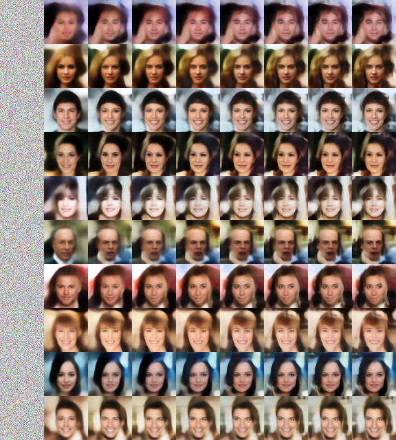
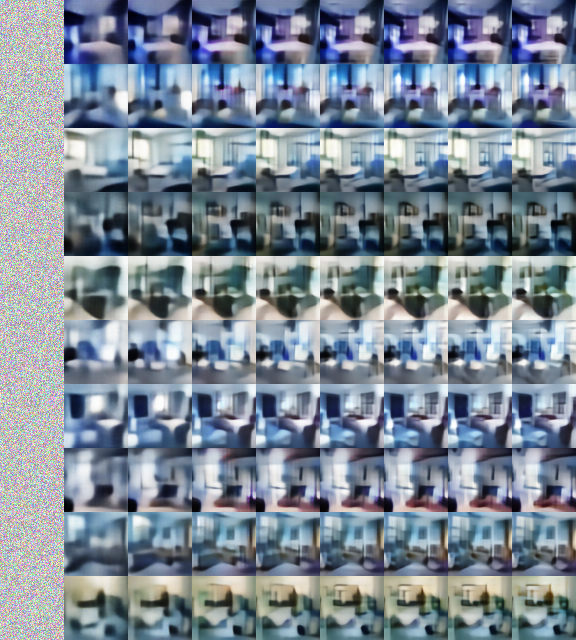
This is the implementation of the Sequential VAE in Towards a Deeper Understanding of Variational Autoencoding Models. The paper identifies a link between power of latent code and sharpness of generated samples. We are able to generate fairly sharp samples by gradually augmenting the power of latent code.
The model is a (non-homogeneous) Markov chain. For each step, we take the results from previous step, learn a new latent code, and train the model to perform reconstruction conditioned on both. We extensively use shortcut/resnet connections so that result from previous step can be well preserved. Samples look like this
For CelebA download the dataset from http://mmlab.ie.cuhk.edu.hk/projects/CelebA.html
Download the aligned and cropped version, unzip into a folder, and pass the path of that folder as db_path argument. Note that your db_path folder should directly contain all the image files without any additional nesting. You folder should look like this
Now you can train by running
python main.py --dataset=celebA --db_path=/path/to/celebA/dataset
You can see the visualizations in the folder $pwd/models/[network_name]/samples
For LSUN bedroom we provide a preprocessed version available for download here (Google Drive). The images have been center cropped, resized, and organized into batches with 10000 images each for efficient I/O.
Download this dataset, unzip into a folder. This folder should also directly contain all the npy files without additional nesting. You can train by running
python main.py --dataset=lsun --db_path=/path/to/lsun/dataset
For other LSUN scene classes you should first preprocess the files into batches of 10000, where each batch is a numpy array [batch, height, width, channel]. Place these batches into the db_path folder.
- To use a particular GPU/GPUs add option
--gpus=[ids]such as--gpus=0,1to use GPU 0 and 1. The visualizations in the paper are produced after 2 days of training on a single Titan X. - To use other architectures other than default, use
--netname=[name]. For supported architectures please refer to code. The name is the unique identifier for the network, and all related training log, visualizations, and checkpoint files, etc will be stored in the directory$pwd/model/netname. For example, to run visualization with tensorboard usetensorboard --logdir=[that directory] - To also visualize the training process with a GUI window add
--use_gui. By default all plots will be stored to network directory, this will also plot them in a window in addition to that. - To change batch size, add
--batch_size=[size] - To visualize and plot the autoencoding reconstruction of the model, add
--plot_reconstruction - To add Gaussian and salt and pepper noise to perform denoise training add
--denoise_train - To control the number of batches before we visualize and make plots, use
--vis_frequency=[num_batch]
The baseline architecture used is the Variational Ladder Autoencoder
This model can be viewed as a generalization of Infusion training. The difference is that for each time step we explicitly learn a latent code rather than using random pixels from ground truth as latent code.


