Intended to introduce students into the world of electrochemical research going on in the School of Engineering, Macquarie University. The methods will be added as soon as decently written packages become available in the group.
Time-resolved electrochemical method allowing for the direct observation of surface electron transfer in heterogeneous electrochemical systems. The full description of the method is given in the paper https://pubs.acs.org/doi/abs/10.1021/acs.analchem.1c01286
Installation: Simply load zip archive from Github, extract and open folder "ElectrochemLabUtils" in VSCode.
Example usage:
import os
import numpy as np
import VFSWV_read_and_plot as VFSWV

# electrode size
e_size = 1.0

# location of the SWV files:
current_script_location = os.path.dirname(__file__)
data_folder_name = "Example_data\CoPc_VFSWV_txt_data"
directory_to_process = os.path.join(current_script_location, data_folder_name)

# create arrays of step delay times (ms) and frequencies (Hz)
step_times = np.array([0.4, 0.6, 0.8, 1.0, 1.2, 1.4, 1.6, 1.8, 2.0, 2.2, 2.4, 2.6, 2.8, 3.0, 3.2, 3.4, 3.6, 3.8,
                    4.0, 4.2, 4.4, 4.6, 4.8, 5.0, 5.4, 5.8, 6.2, 6.6, 7, 7.4, 7.8, 8.2, 8.6, 9, 9.4,
            9.8, 10.2, 10.6, 12.8, 13.6, 14.4, 15.2, 16, 17, 18, 19, 20, 22, 24, 26, 28, 34, 38, 42, 46, 50, 55,
                    60, 65, 70, 75, 80, 85, 90, 95, 100, 125, 150, 175, 200, 300, 400, 500, 750, 1000, 1500])
frequencies = 500/step_times

# define a window of interest across x and y axis
e_boundary_highest, e_boundary_lowest = 0, -0.9
log_frequency_highest, log_frequency_lowest = 3.09, -0.47

# produce the linearly spaced arrays for interpolaiton and plotting
e_new = np.linspace(e_boundary_highest, e_boundary_lowest, 100)
freq_new = np.linspace(log_frequency_highest, log_frequency_lowest, 100)


# generate the experimentally recorded 2D VF-SWV and make the linealry spaced 2D arrays for plotting
x, y = np.meshgrid(e_new, freq_new)
sq_w_v = VFSWV.extraction_of_swv(path=directory_to_process,
                            experimental_frequencies=frequencies,
                            array_of_frequencies_for_plotting=freq_new,
                            array_of_potentials_for_plotting=e_new,
                            size_of_electrode=e_size,
                            dlc_correction=False)

# plot the experimental data and preview only
VFSWV.plot_2D(x=x,
        y=y,
        z=sq_w_v,
        figure_name=None)

VFSWV.plot_3D(x=x,
        y=y,
        z=sq_w_v,
        figure_name=None)

# save figures
# figure_export_dir = os.path.join(current_script_location, 'Example_plots')
# VFSWV.plot_2D(x=x,
#         y=y,
#         z=sq_w_v,
#         figure_name=figure_export_dir + "/CoPc_CNT_2D_graph")

# VFSWV.plot_3D(x=x,
#         y=y,
#         z=sq_w_v,
#         figure_name=figure_export_dir + "/CoPc_CNT_3D_graph")
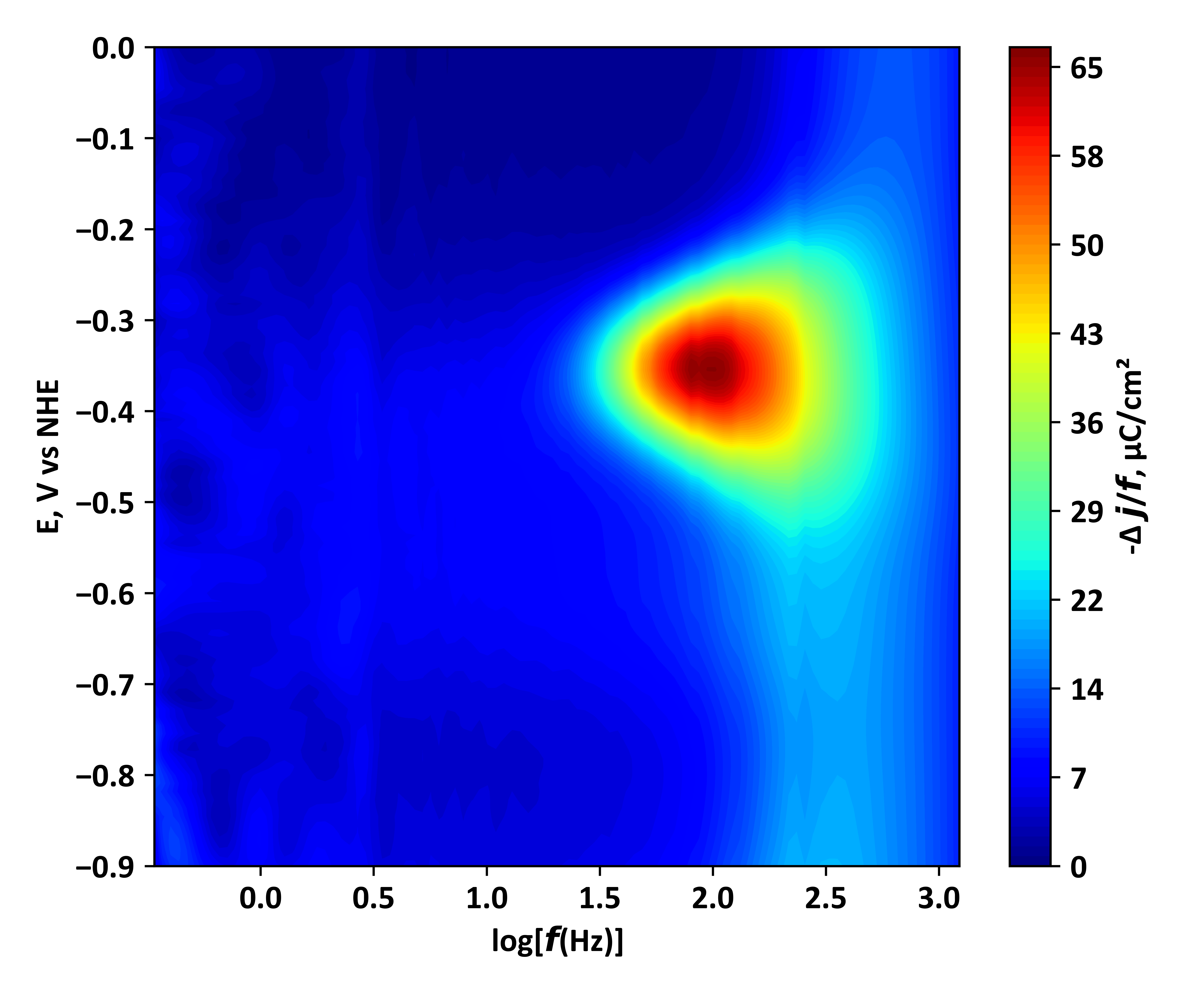
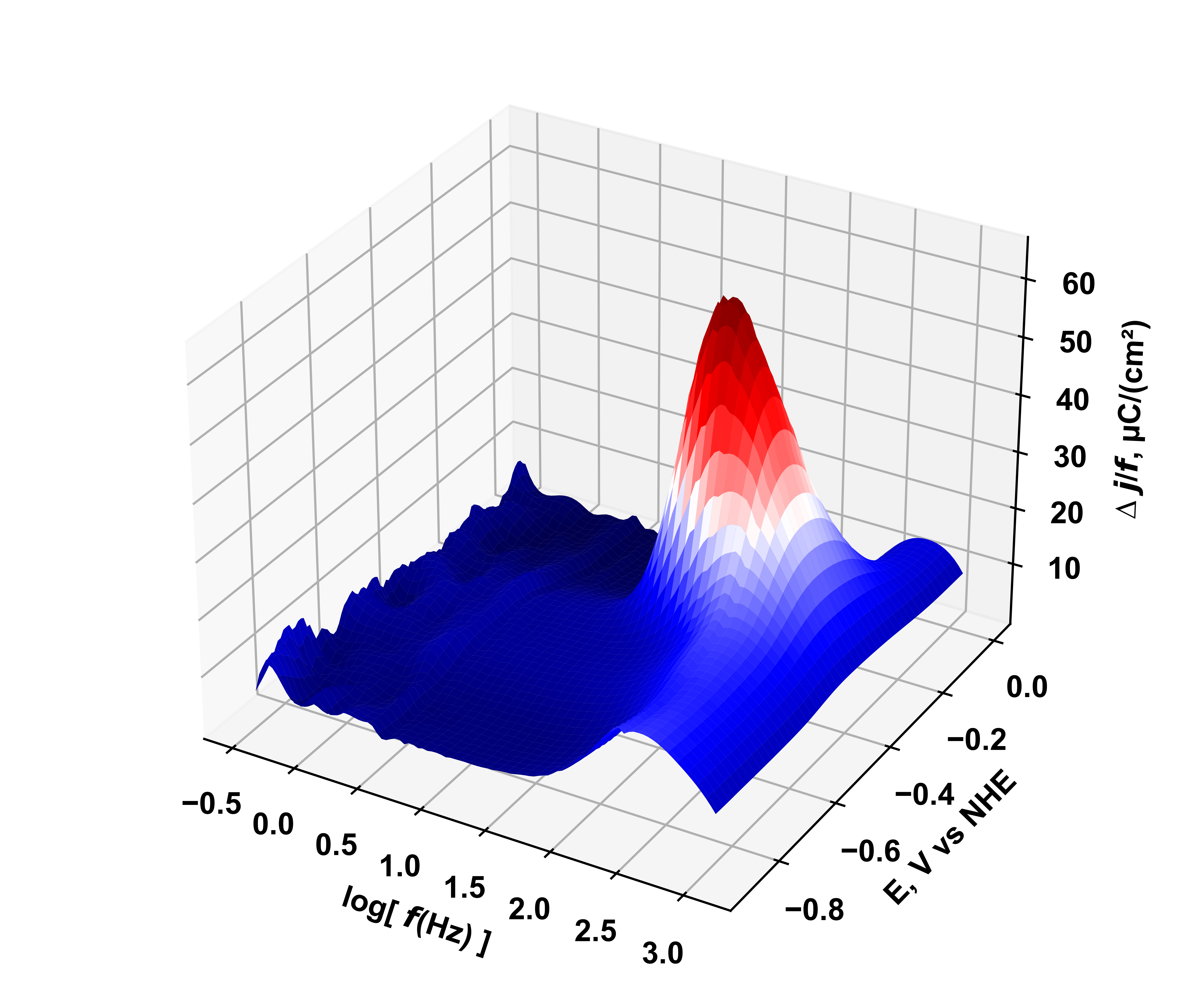
Example output and short interpretation:
VF-SWV analysis of CoPc/CNT composite:
The main peaks correspond to a relatively fast 1e transfer process taking place of the surface. The additional wide band stretching across the entire frequency domain arises due to the contribution of non-faradic currents.

