traceR

traceR allows you to click on an image in the plot window (kind of like a join the dots picture) and record the coordinates into a data frame. They can then be plotted independently in a ggplot.

This enables the user to plot custom shapes in R without having to manually enter the coordinates into a data frame.

Installation

Install from Github:

devtools::install_github("doehm/traceR")

Usage

TL;DR

To use trace_image:

Plot an image in ggplot
Run df <- trace_image()
Click on the desired coordinates in the required sequence
When finished click on the left side of the plot window between 0 and stop_window pixels on the x-axis
Inspect the coordinates with inspect_trace

The coordinates are scaled to (0, 1) by default and returned as a tibble. There is an option to return the raw pixel coordinates by setting scale = FALSE. You will want to do this if you are selecting multiple layers or objects.

Example

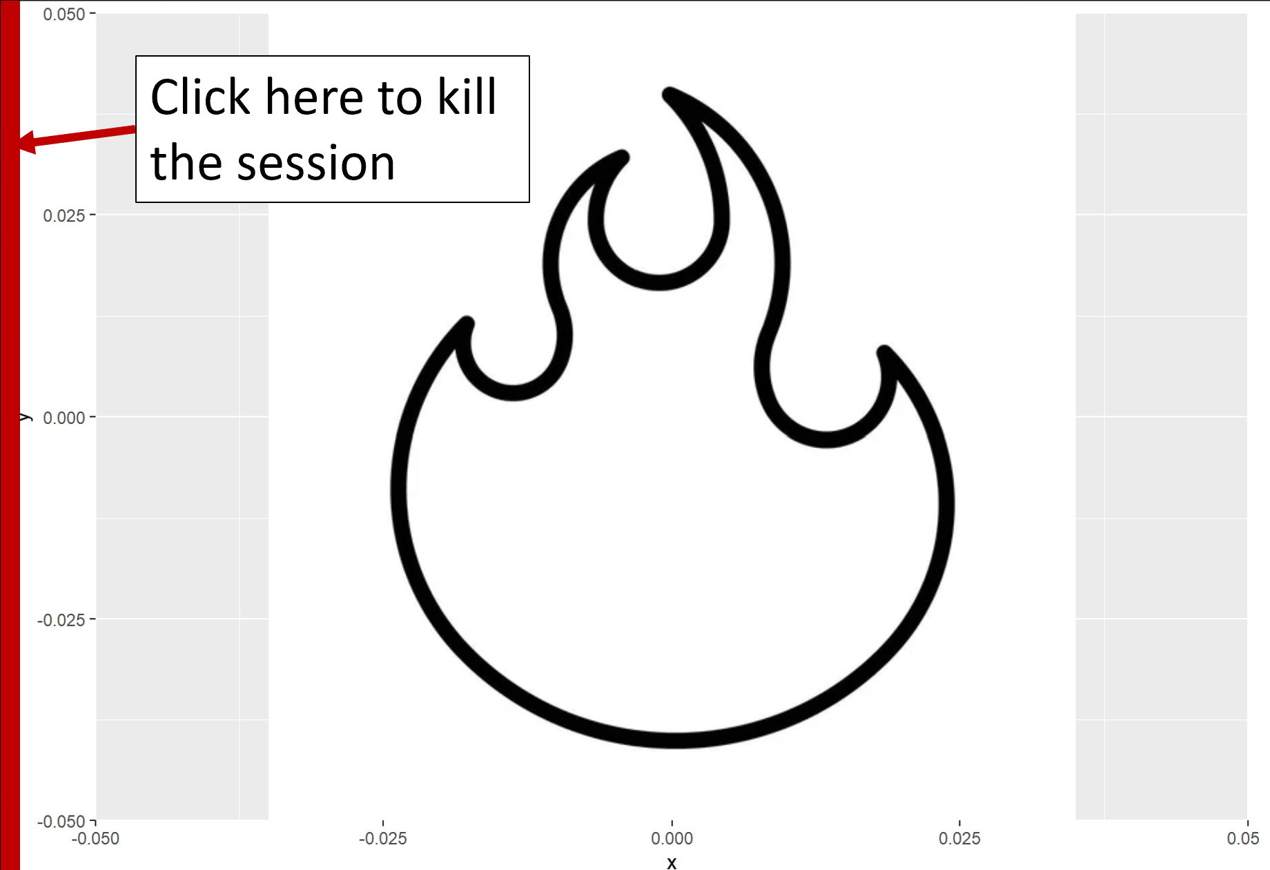
To demonstrate with a more detailed example, suppose you really liked the design of this flame and wanted to use it for some data viz.

Firstly, plot the flame with ggplot2.

library(tidyverse)
library(ggpath)

flame_path <- "https://github.com/doehm/traceR/blob/main/dev/images/simple-flame.jpg?raw=true"
ggplot() +
  geom_from_path(aes(0, 0, path = flame_path))

Then run

df_flame <- trace_iamge(scale = TRUE)

Some info will pop up in the console and you are ready to record the coordinates. Start anywhere on the outline of the image and click and suitable intervals. For tighter curves you’ll want to shorter intervals to better recreate the curve.

Click twice for sharp points like at the peak of the flames. ggforce::geom_bspline_closed0() is great at interpolating the points and drawing a curve and we can trick it into drawing a sharp point by clicking in the same place twice.

Click on the left side of the plotting window when you are done recording the coordinates (within 0-20 pixels by default). This will kill the recording and return the data frame.

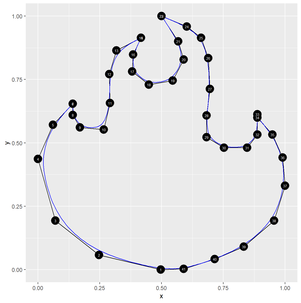
Inspect the coordinates with inspect_trace(). This plots the coordinates using geom_polygon() and geom_bspline_closed0 so you can see if you got what you need.

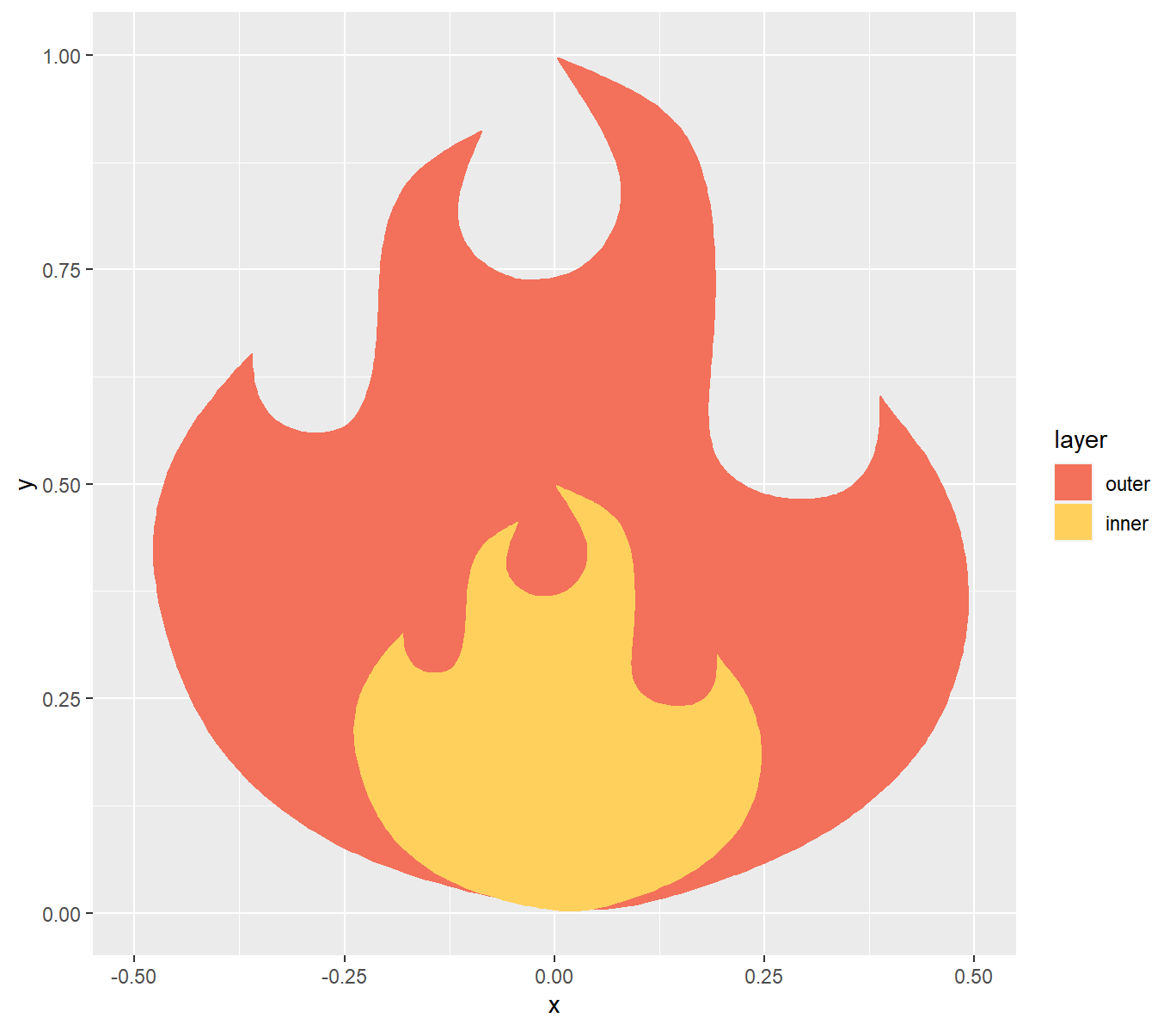
inspect_trace(df_flame)

Now that you have what you need as a data frame you can plot it using standard ggplot2 geoms. For example

pal <- c(outer = '#f3705a', inner = '#ffd15c')

df_flame1 <- df_flame |> 
  mutate( # create the outer layer
    x = x-0.5, # center the coords around 0
    layer = "outer"
    ) |> 
  bind_rows( # create and append the inner layer
    df_flame |> 
    mutate(
      x = (x-0.5)*0.5, # center and scale the coords by 50%
      y = y*0.5,       # scale the coords by 50%
      layer = "inner"
    )
  ) |> 
  mutate(layer = factor(layer, levels = c("outer", "inner")))

df_flame1 |> 
  ggplot(aes(x, y, fill = layer)) +
  geom_bspline_closed0() +
  scale_fill_manual(values = pal)

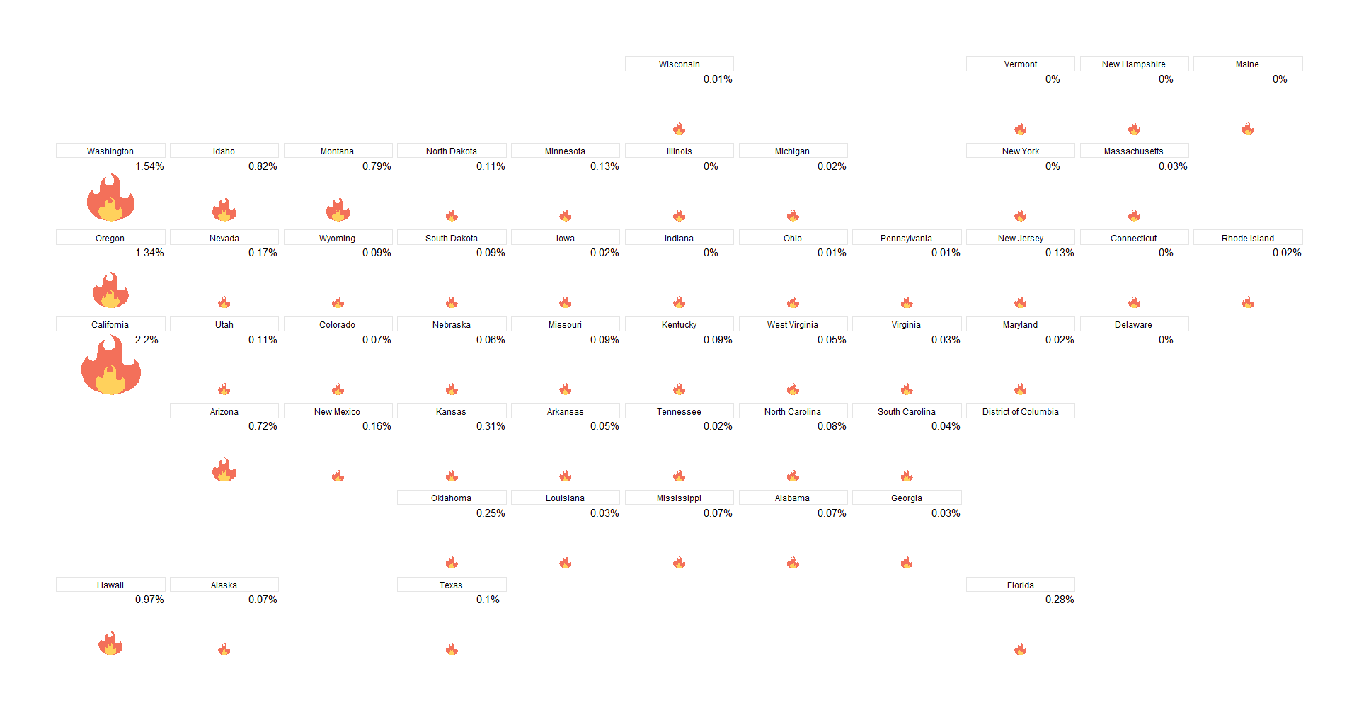
At this point you can get creative and do what you want with it. For example you could use the flame to create an infographic of bushfire damage in the US.

library(geofacet)

# scale the coords for each state based on the total area burned
df_bushfires <- read_rds("https://github.com/doehm/traceR/blob/main/dev/data/bushfires.rds?raw=true")

df_base <- map_dfr(df_bushfires$code, ~{
  dat <- df_bushfires |>
    filter(code == .x)
  df_flame1 |>
    mutate(
      x = x*dat$cat_burned,
      y = y*dat$cat_burned,
      code = dat$code,
      state = dat$state
    )
})

df_base |>
  ggplot() +
  geom_bspline_closed0(aes(x, y, fill = layer), colour = NA) +
  facet_geo(~state, grid = "us_state_grid1") +
  scale_fill_manual(values = pal) +
  xlim(-4, 4) +
  theme_void() +
  theme(
    plot.margin = margin(t=60, b=60, l=60, r=60)
    legend.position = "none",
    strip.background = element_rect(colour = "grey90"),
    strip.text = element_text(margin = margin(t = 3, b = 3))
  )

It’s not perfect but it is a very convenient way to get the coords into a data frame for you to start working with.

This flame is simple enough that you wouldn’t need to trace it to use it in this way. But if you have a more complex image with a bunch of stuff going on it comes in handy.

Once you start getting creative you can layer up traces and create images like this cute little dino that I’ve adopted for the hex!