This repository contains data collection, cleaning and analyses of air quality data of Beijing from 2013-2017. We used the data from twelve sites located in around Beijing's city center.
We downloaded and curated data from the University of California - Irvine. The data set was provided by the authors of 'Cautionary Tales on Air-Quality Improvement in Beijing' (2017), a paper published in Proceedings of the Royal Society.
For this project, we aim to analyze the sampled particulate matter from the twelve testing sites in Beijing in order to identify key trends and predict the levels of PM 2.5 (particulate matter with a circumference of 2.5 microns).
This is small particulate matter that can be suspended in the air for long periods of time before it enters the lungs.
First, we moved to combine all of the twelve sites into a single dataset interpolating the data.
We tested for stationarity and whether there was correlation between the features and time periods throughout our dataset.
Next, we began to fit models in an effort to prepare our models to predict the last twenty percent of the data that we had set aside as a test case.
Due to the time constraints and large amount of data, we decided to focus on a univariate time series forecast vs a multivariate time series forecast. One reason for the switch was that our hardware was unable to keep up with the amount of observations and features in an hourly prediction with multiple feature.
- PNG -- contains images created during EDA and those linked in README
- 001_Data_Cleaning.ipynb -- contains all processes that went into cleaning the time series
- 002_EDA.ipynb -- creates the visuals and shows analysis of those visuals for the project
- 003_Modeling.ipynb -- contains forecasting models against holdout data
- README.md
-
Marking a Target/Identifying Stakeholders
- To whom does it matter if we can predict the amount of particulate matter in the air?
- Residents of an Area and Tourists:
Will they be able to enjoy time outdoors? - People Who Suffer From Respiratory Illnesses:
Will their conditions worsen? Do they have to worry about loved ones contracting the same illness if not already predisposed? Will this contribute to premature death?
- Residents of an Area and Tourists:
- To whom does it matter if we can predict the amount of particulate matter in the air?
-
Understanding how different countries and regions may battle against the proliferation of particulate matter
- Are some regions experiencing a rise in PM 2.5 while others are experiencing a decrese?
-
Understanding the viability in different models
- Is it better to use a Facebook Prophet or a basic ARIMA?
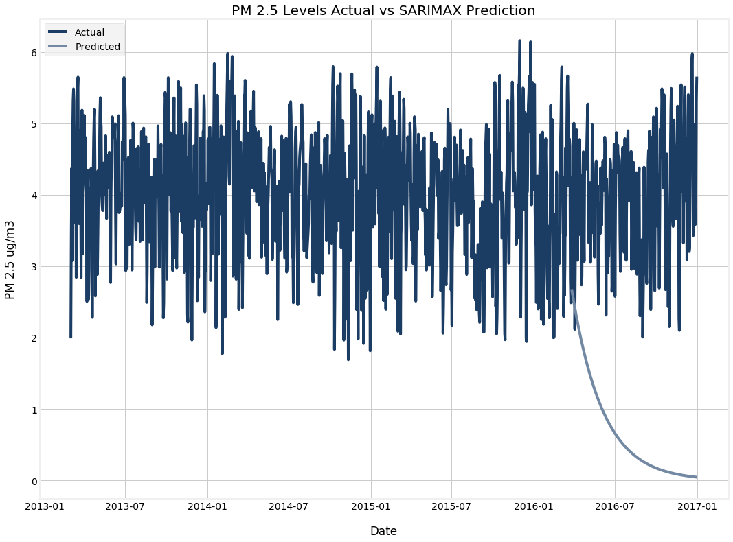
- Will SARIMAX models work with this data set?
- Does the best model do a good job of predicting the target levels?
Before we dive deeper into the questions, here is some information on our data.
- The data is focused on 12 testing sites in and around Beijing's city center from 2013-2017.
- The data here was downloaded from The University of California - Irvine Machine Learning Repository.
- You can find the dataset and dictionary here.
Now we will briefly discuss what our dataset contains.
With targeting particulate matter floating in the air, we explored how to better predict the target variable to make a better model for our stakeholders.
The data was capped at the last day of December 2016. While the data extended into 2017, it only covered the first two momnths and the predictions would have been affected if we allowed an entire year to be represented by the two coldest months of winter. For the purpose of this study, we have decided to work with the daily mean value of PM 2.5 vs the hourly reading. This was done to make a more strenuous deadline. While the data is numerous, the hardware cannot handle the large amount of observation (almost 500 thousand) and features.
Doing each of the stations individually would not have been a cost effective project. So instead, we elected to aggregate the data from the twelve sites and forecast the city of Beijing as a whole.
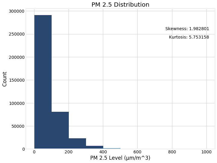
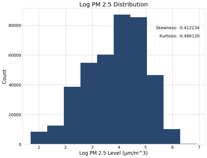
Our first step was to examine the distribution. We found that it was not normally distributed.
So we natural log transformed it. It took on the shape of a normal distribution.
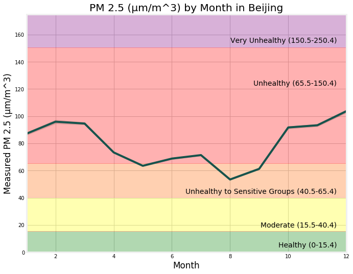
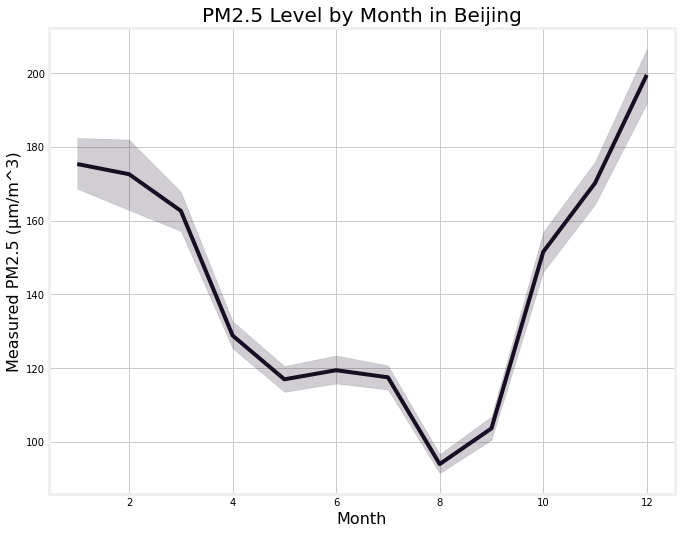
First, the breakdown of PM 2.5 on Monthly Averages for Beijing.
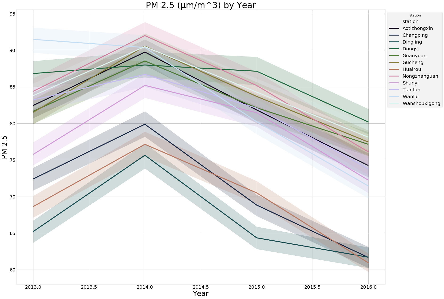
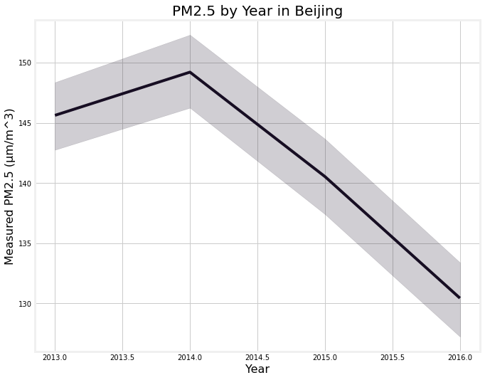
Secondly, the breakdown of PM 2.5 on Yearly Averages for Beijing.
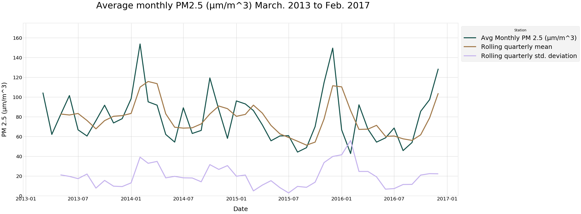
Finally, the visual of the rolling summary statistics.
Using a continuous variable means that we want to use RMSE as our target metric. Our goal is to minimize RMSE because it is the count of our residuals and will help us determine where our predicted values fall around the actuals.
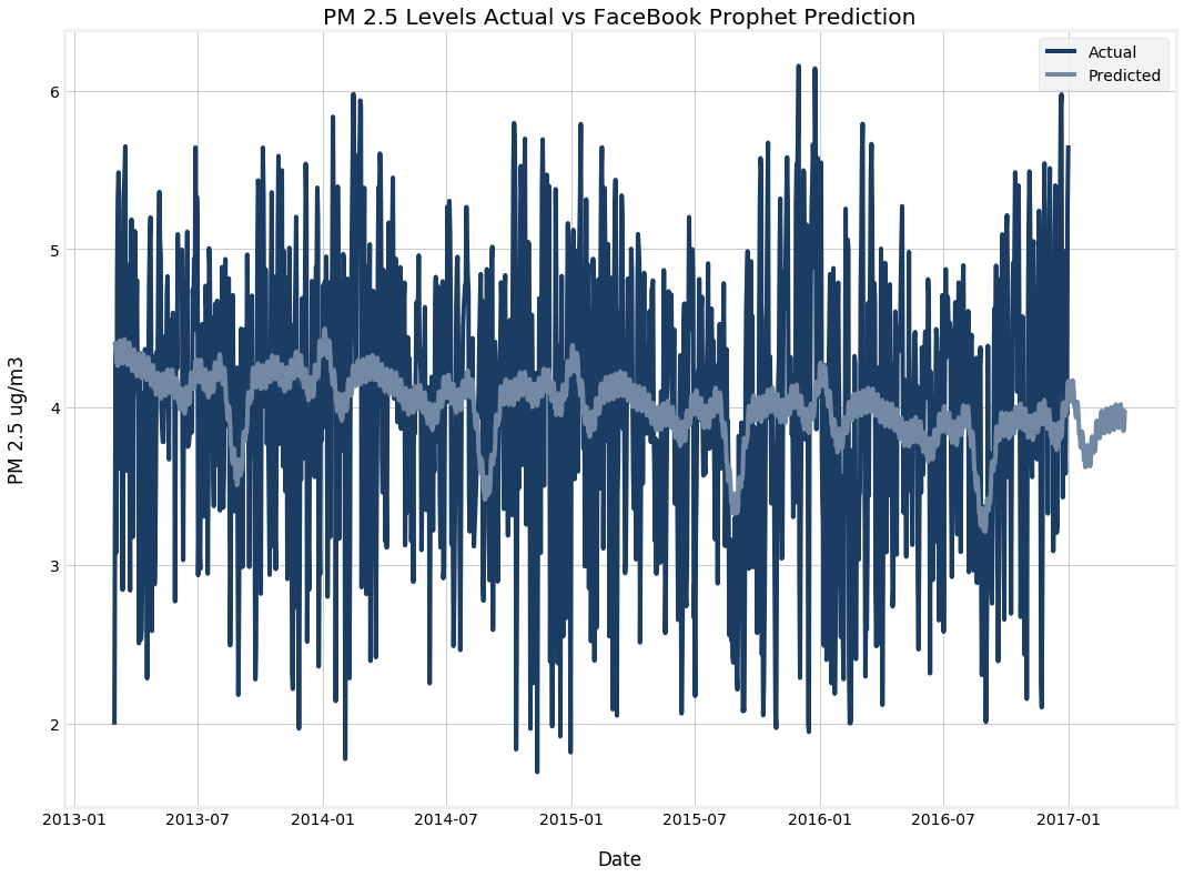
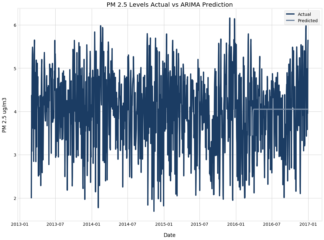
We ran several models, including a dummy model that ran the average of the test set, the ARIMA Model, and the SARIMAX Model.
| Model | RMSE |
|---|---|
| ARIMA | 0.80272 |
| SARIMAX | 3.5193 |
| FB Prophet | 0.97109 |
RMSE: 0.97109
RMSE: 0.80272
RMSE: 3.5193
Our models performed admirably considering the limitations of our hardware. Aggregating the data into a daily city-wide observation led to a lot of the data being lost. Without a concrete way to weigh each station, we were forced to consider them all equally.
In our ARIMA specification, the middle number in both the first and the second bracket is zero. That means, there is no simple differencing and no seasonal differencing. Thus our series appears to be mean-stationary (rather than integrated or seasonally integrated). (The AR and MA parameters yielded by the auto.arima function are restricted to be in the region of stationarity; meanwhile, nonstationarity can be introduced by simple or seasonal differencing.) Given a mean-stationary process, you should actually expect the point forecasts to converge to the mean of the process. That is one of the intrinsic features of a mean-stationary time series. And that is also why these kind of processes are called "mean-reverting".
We would like to run further tests on datasets individually. Breaking down the data set by testing site would give us access to more accurate data.
As it stands, the aggregated data yielded a pretty strong model. Our ARIMA model had an RMSE score of 0.77 compared to the mean score of 3.955, the predicted values were not far off.
Facebook Prophet had an RMSE score of 0.971 and an MSE of 1.005 which wasn't far from ARIMA, but short term predictions may have been even better and more accurate.
In terms of the models used, we want to explore neural networks in more detail and the expanded use of FaceBook Prophet.
-
Increasing transparency of testing site for public distribution & consumption
-
Keeping residents informed on progress showing air quality is a viable short term goal
-
Public health campaigns to discourage use of transportation that rely on fossil fuels and focus on green public transportation
-
Using the data provided by the sites to track increases in smog causing pollutants would helping environmentalists recognize increasing pollution trends and resolving problems quickly.
