Body Composition Assessment Dataset

This repository contains the data and code for the works

"Artificial Intelligence to Assess Body Composition on Routine Abdominal CT Scans and Predict Mortality in Pancreatic Cancer – A Recipe for Your Local Application", European Journal of Radiology (2021)
"Fully Automated AI Body Composition Quantification from Abdominal CT Scans - Training Data, Model Code and Trained Weights", Data in Brief (2021)

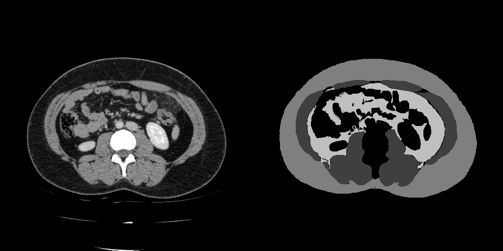
Overall, we annotate 40 studies from the publicly available LiTS Dataset on slices at the level of L3 vertebrae, and learn models to automatically assess body composition.

Due to the large file sizes, the models and the data are not tracked by git and will have to be downloaded with the following instructions.

Prerequisites

Linux (Ubuntu 16.04 tested)
Python 3.7+
Nvidia GPU (cuDNN 8.0 and CUDA 11.0)

Getting Started

We will walk you through some simple steps to run inference with our trained weights and an example LiTS study.

Clone this repository.

git clone https://github.com/stmharry/body-composition.git && cd body-composition

Download models and an example CT.

# Copy and paste this command to your command line
curl https://body-composition.s3.amazonaws.com/models.tar.gz | tar -zx -C .
# or if you feel lazy, use the pre-packed command
make pull-model

Install required packages. (or use virtual environment)

# Setting up virtual environment (optional)
virtualenv -p python3.7 venv && source venv/bin/activate
# or if you are using conda
conda create -n venv python=3.7 && conda activate venv && conda install pip
# pip install
pip install -r requirements.txt

Run the model prediction on the example CT and collect outputs at ./results.
```
make STAGE=first && make STAGE=second
```

By this point, you should expect a new directory results with this file hierarchy:

results
├── first
│   ├── 1014-2.nii.gz
│   ├── ... 
│   ├── 1014.pdf
│   ├── 1014.png
│   ├── all.pdf
│   └── stat.csv
└── second
    ├── 1014-2.nii.gz
    ├── 1014-2.pdf
    ├── 1014-2.png
    ├── ... 
    ├── all.pdf
    └── stat.csv

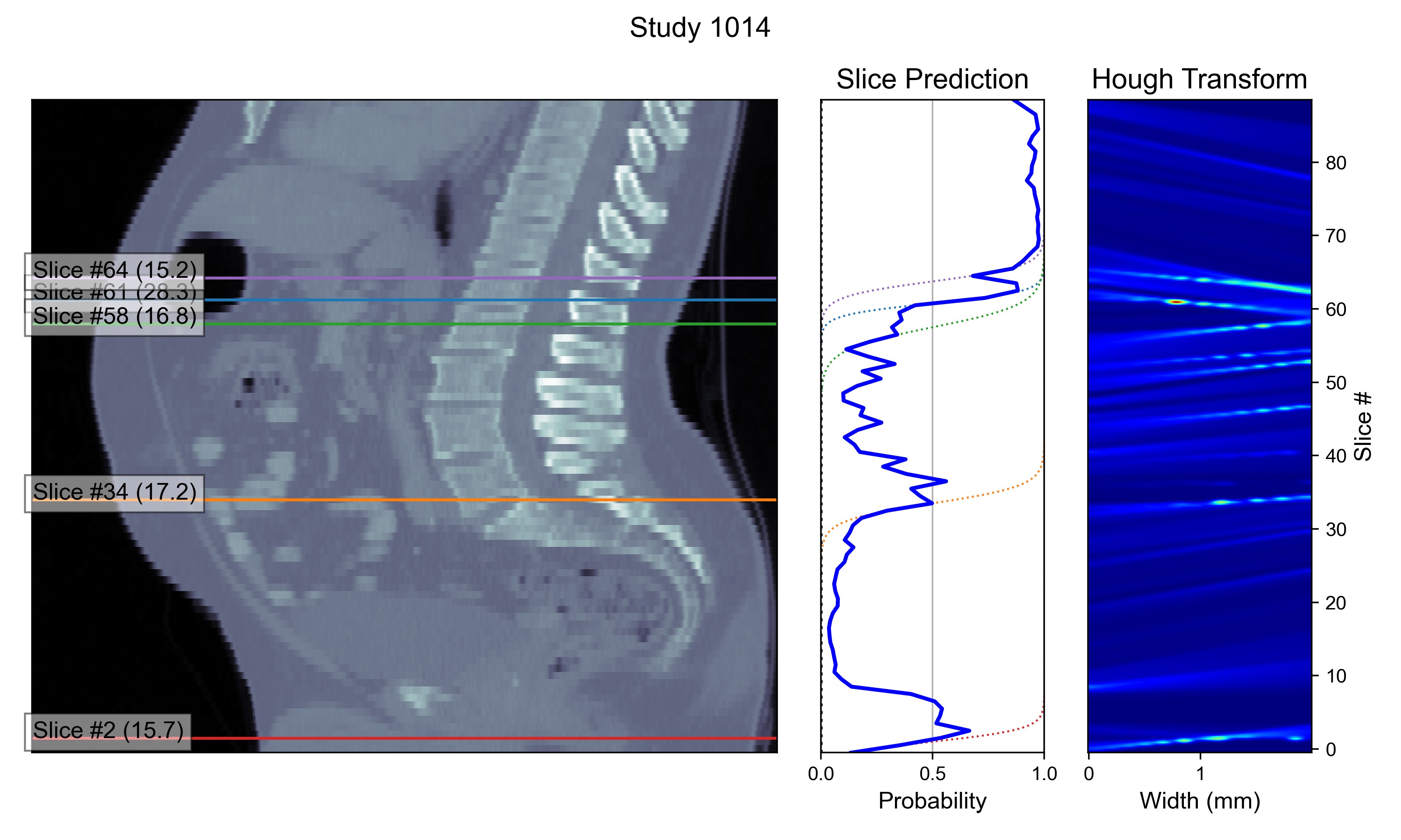
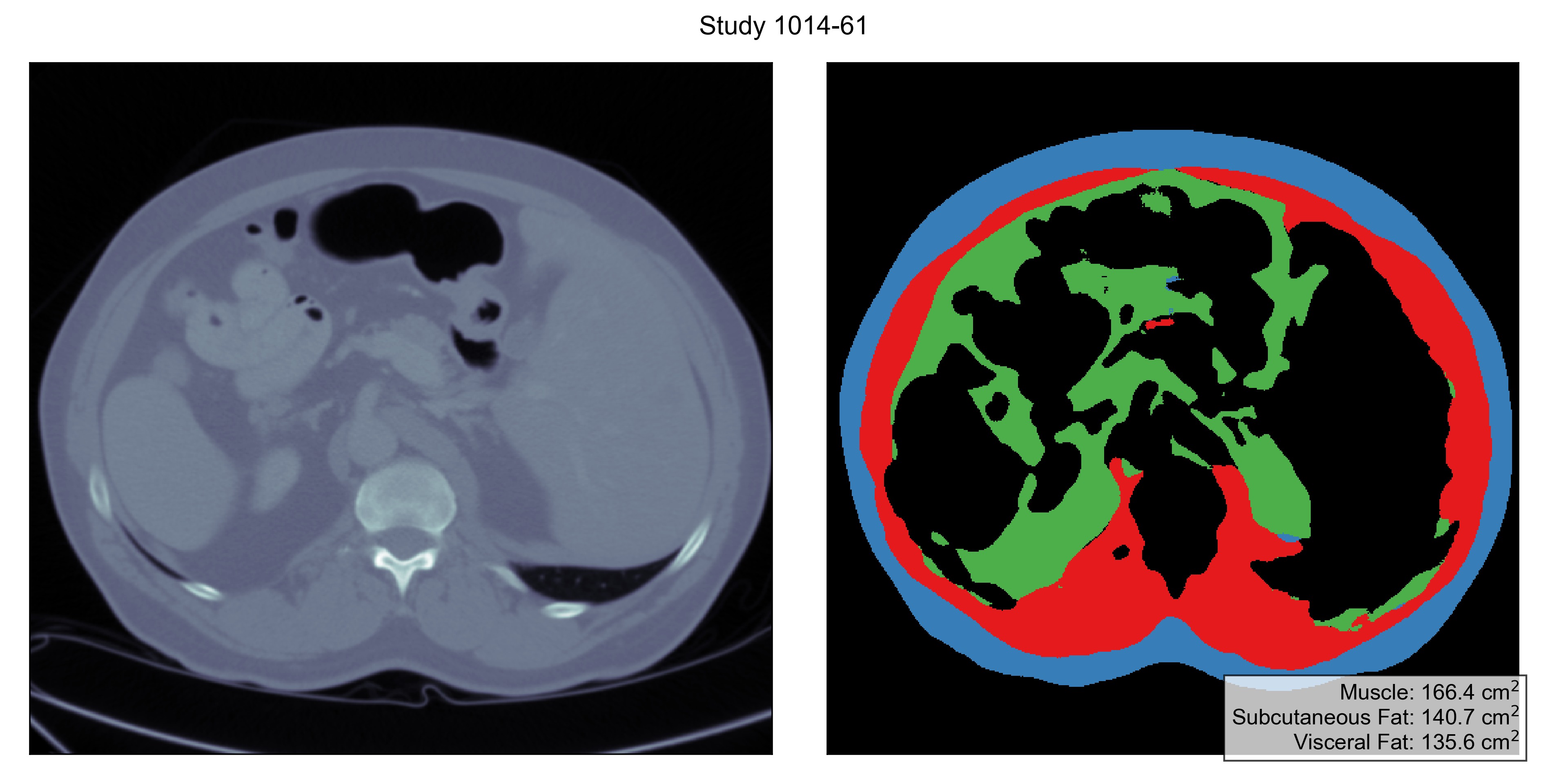
The folder results/first contains inference results for the first stage of the model which detects the L3 vertebra, and results/second performs second-stage analysis on each of the proposed slice. Example outputs are shown as follows:

The Data

The Liver Tumor Segmentation Challenge released 200 CT scans in total, from which we select 29 training studies and 12 test studies for annotation. To fetch the data, run

# Copy and paste this command to your command line
curl https://body-composition.s3.amazonaws.com/data.tar.gz | tar -zx -C .
# or if you feel lazy, use the pre-packed command
make pull-data

In data/studies, you can find raw studies (in NIFTI .nii.gz format) that we have annotated, and in data/masks, the per-pixel annotation (also in NIFTI format). Each study has a slice labeled with three tissue types:

Muscle (label 1),
Subcutaneoue Fat (label 2), and
Visceral Fat (label 3).

Using Your Own Data

Inference

It is straightforward to use your own CT data for inference. Simply create volumes in NIFTI format with the voxels in RAS+ orientation and a shape of [512, 512, slices] where slices can be arbitrary. Place this study under data/studies and rerun ./predict.sh, and you can extract the corresponding inference results in results.

Training

To prepare data for training, it is one more step than placing the files in data/studies: you also have to assign them into either the training set or the evaluation set. In files data/splits/first/{train,eval}.txt you should add the names of your study depending on the data split you wish to put them into. These two files are for training/evaluating the first stage, and the same process goes similarly for the second stage where you would modify data/splits/second/{train,eval}.txt.

To kick off training with the new training splits, run the following commands to train two stages respectively:

# Training the first stage
make DO=train_eval STAGE=first
# Training the second stage
make DO=train_eval STAGE=second

New models will be saved in models/<some-fancy-timestamp>, and you can use tensorboard to monitor the training process with tensorboard --logdir models.

Reference

For any question, please contact Tzu-Ming Harry Hsu.

doumeng/body-composition