Adaptive Wiener Loss

Data comparison lies at the heart of machine learning: for many applications, simplistic loss functions - such as the L2 loss that rely on local element-wise differences between samples - have taken preference. Such metrics are notorious for producing low-quality results. The proposed Adaptive Wiener Loss (AWLoss) addresses this issue by introducing a new convolutional approach to data comparison; one that uses a Wiener filter approach to naturally incorporate global information and promote spatial awareness within the compared samples.

This repository contains an implementation of this loss in a natural Pytorch as here it is promoted as a loss function to drive deep learning problems. The source code is a single file that contains a single class named AWLoss. Its usage and customisation are described below.

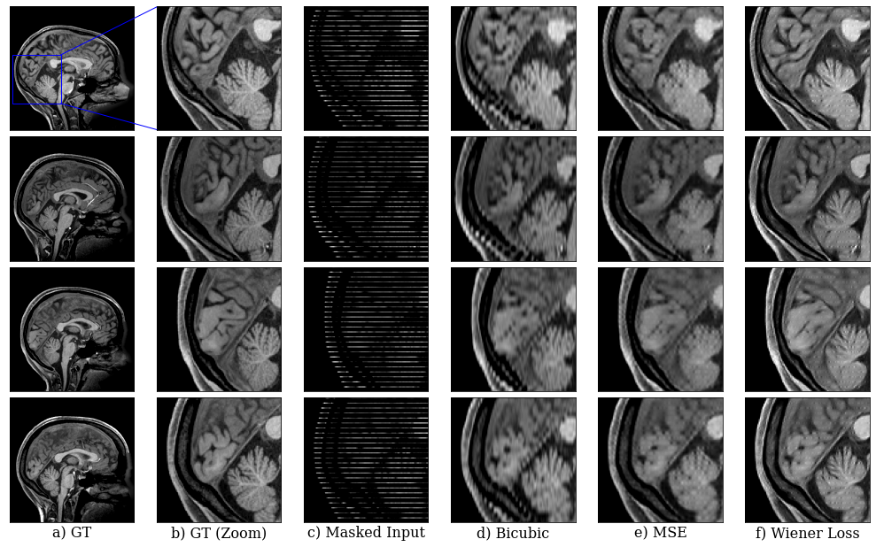
A demonstration of this loss in a deep learning context is shown in the following figure for a medical data imputation problem:

In the figure, (e) and (f) are obtained through the training of a UNet.

Installation

git clone https://github.com/dpelacani/WienerLoss.git
cd WienerLoss

# create conda environment (recommended)
conda create --name wiener
conda activate wiener

# install dependencies
pip install -r requirements.txt

# for running examples and performance notebooks
pip install -r requirements-optional.txt

# install package
pip install -e .

Example usage

import torch
from wiener_loss import WienerLoss

wiener_loss = WienerLoss()
x = torch.rand([1, 3, 28, 28])
y = torch.rand([1, 3, 28, 28])

wiener_loss(x, y)
>> tensor(1.4073, grad_fn=<DivBackward0>)

wiener_loss(x, x)
>> tensor(0., grad_fn=<DivBackward0>)

Method Overview

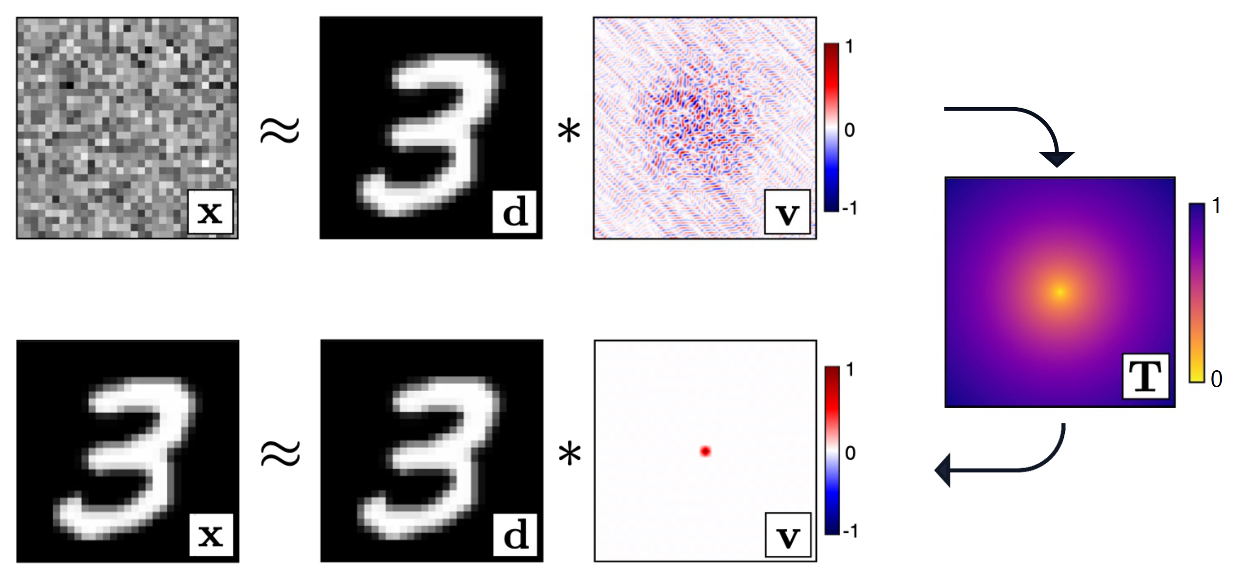
The main idea behind this comparison method, firstly introduced by Warner and Guasch (2014), is that two signals are considered identical when their corresponding matching filter is an dirac delta at zero lag (i.e. convolutional idendity). We start by considering two signals, $\mathbf{x}$ and $\mathbf{d}$, that are not identical. A convolutional Wiener filter $\mathbf{v}$ that provides the best least squares match between the two samples is computed by the well known equation:

$$ \mathbf{v} = (\mathbf{D}^{T} \mathbf{D})^{-1} \mathbf{D}^{T} \mathbf{x} $$

where $\mathbf{D}$ is the Toeplitz matrix of signal $\mathbf{d}$ that achieves a convolution operation in matrix form.

We then act on this filter through an arbitrary a penalty function $\mathbf{T}$ that rewards energy at zero lag, and monotonically penalises energy at non-zero lags:

$$ L = \frac{1}{2}||\mathbf{T} * (\mathbf{v} - \mathbf{\delta)}||^{2}_{2} $$

By minimising $L$, we implicitly drive signal $\mathbf{d}$ to become more similar to signal $\mathbf{x}$

Input Arguments

On object initialistion:

Args:
    method, optional
        "fft" for Fast Fourier Transform or "direct" for the
        Levinson-Durbin recurssion algorithm. Defaults to "fft"
    filter_dim, optional
        the dimensionality of the filter. This parameter should be
        upper-bounded by the dimensionality of the data. If data is
        3-dimensional and filter_dim is set to 2, one filter is computed
        per channel dimension assuming format [B, NC, H , W]. Current
        implementation only supports filter dimensions for 1D, 2D and 3D.
        Defaults to 2
    filter_scale, optional
        the scale of the filters compared to the size of the data.
        Defaults to 2
    reduction, optional
        specifies the reduction to apply to the output, "mean" or "sum".
        Defaults to mean
    mode, optional
        "forward" or "reverse" computation of the filter. For details of
        the difference, refer to the original paper. Default "reverse"
    penalty_function, optional
        the penalty function to apply to the filter. If None, a Gaussian
        penalty will be created of mean zero and standard deviations
        specified below. Mutually exclusive with "std". Default None
    store_filters, optional
        whether to store the filters in memory, useful for debugging.
        Option to store the filers before or after normalisation with
        "norm" and "unorm". Default False.
    epsilon, optional
        the stabilization value to compute the filter. Default 1e-4.
    std, optional
        the standard deviation value of the zero-mean gaussian generated
        as a penalty function for the filter. If 'penalty_function' is
        passed this value will not be used. Default 1e-4.

On object calling

Args:
    recon
        the reconstructed signal
    target
        the target signal
    epsilon, optional
        the stabilization value to compute the filter. If passed,
        overwrites the class attribute of same name. Default None.
    gamma, optional
        noise to add to both target and reconstructed signals
        for training stabilization. Default 0.
    eta, optional
        noise to add to penalty function. Default 0.

Note on Filter Dimensions

The AWLoss class supports data of dimensions up to 3, excluding the batch dimension. The filter dimension can be arbritarily chosen by the user, up until the dimension of the data itself, i.e. a 1D signal cannot be processed using filter_dim as to 2 or 3, but a 3D signal can be processed processed using filter_dim as 1, 2 or 3.

Using the 1D version of the AWLoss flattens the signal before evaluation in all dimensions apart from the batch dimension; in the 2D implementation, a single 2D filter is computed for each channel of the data; and in 3D a single 3D filter is calculated using the number of channels as the third dimensionality.

Further improvements to this code will allow dimensions up to 4, where the first dimension is the number of channels and the following 3 are the volumetric data. In such, this would calculate one 3D filter per channel in the signal.