Legislative Voting Data
Motivation
I originally started thinking about this data while working on this paper in 2016: A Random Dot Product Model for Weighted Networks joint with Dan Rockmore, where we detected the party structure in the US Senate using an inference technique associated to dot product networks. Recently, I revisited this idea with David Wu and David Palmer at MIT, as an application of a more complex method for tackling the same problem: Bayesian Inference of Random Dot Product Graphs via Conic Programming. A natural follow up question is attempting to apply this method to legislatures that have more than two parties. This led me to compare voting data from both houses of the US Congress to voting data from the European Parliament. The main question I am trying to investiage is whether the voting data provides enough structure to recover the party affiliation of the legislators.
Data Sources
I obtained the US voting data from the Voteview site[1], extracting the Member Ideology and Members' Votes datasets for the 115th Congress and the 114th Senate. The Senate data has 100 legislators and approximately 500 votes while the Congressional data has 451 members and over a thousand votes. The European Parliament data comes from a study of voting and twitter behavior documented at the Clarin.si repository. It represents 787 legislators and approximately 2000 votes.
Processing Steps
Some processing needed to be performed for both data sets. The main issue for the US data is that the information about the legislators is stored in a wide format, with rows indexed by the legislator and columns providing their name and party details, while the roll call votes themselves were reported in a long format with one row per vote. The scripts Process_Votes_House and Process_Votes_Senate join these datasets together into a single dataframe with rows indexed by legislator and columns containing both the legislators information, as well as how they voted on each bill. The European Parliament data for the votes was already sorted by the id of the legislator, so it was simply a matter of appending the relevant party information to the voting data. This is performed in Process_Votes_EP notebook.
In addition to combining the information about the legislators and their respective votes, the vote codes differ significantly between the data sets. The recorded values in the datsets are shown in the following table:
| Data Value | US Congress | Eurpoean Parliament |
| 0 | Not a member at time of vote | For |
| 1 | Yea | Against |
| 2 | Paired Yea | Neutral |
| 3 | Announced Yea | |
| 4 | Announced Nay | |
| 5 | Paired Nay | Unaccounted |
| 6 | Nay | External |
| 7 | Present | Secret |
| 8 | Present | |
| 9 | Abstention |
Visualization
Once I had processed the data, I started to wonder how many votes the average bill received in each of these datasets. For each bill that was considered in each legislative body, I counted the number of affirmative votes (registered as 1s in the US data and 0s in the European data) and made histograms of these values, with the number of votes needed to pass the bill marked in red.
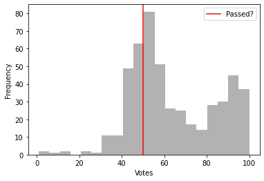 | 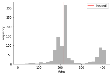 | 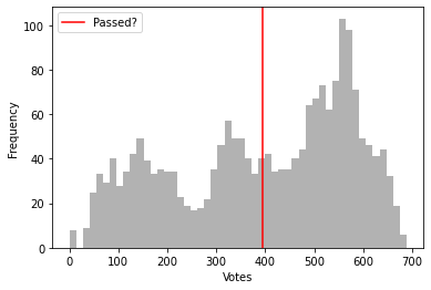 |
| US Senate | US House | European Parliament |
Perhaps unsurprisingly in the US data, many of the bills that actually get voted on are either fairly uncontroversial and very likely to pass or are split along nearly partisan lines and depend on the actions of a few individual representatives. The European Parliament shows a much broader range of voting behavior across the bills that it considers.
Analysis
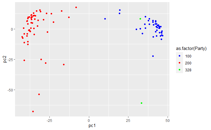
In order to see how much of the party structure could be recovered from the voting data, I used the Hamming distance to compute a dissimilarity matrix for each legislative body and then used MDS to project the data into two dimensions. I then made scatterplots of these embeddings with the nodes colored by the party assignment from the original data. Those figures are shown below and give clear evidence that this is a reliable technique for identifying political structure:
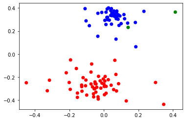 | 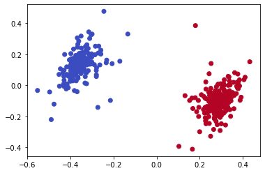 | 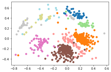 |
| US Senate | US House | European Parliament |
In each case, the dimension reduction technique does place members from the same party close to each other and the clusters are mostly well-separated in the plane (the two representatives marked with green in the Senate data won their seats as independents but both did caucus with the Democratic party). For the European data, I made some additional plots to see what additional structure could be discerned. The left plot shows the same embedding with the legislators colored by the country that elected them, which does not appear to be captured by the MDS procedure. The center plot show a three dimensional projection of the voting data, which does seem to separate some of the parties a little better than the two dimensional version above. Finally, I used the dot product approach from the original paper to generate some networks from the underlying data, which do appear to show clustering by party, as expected.
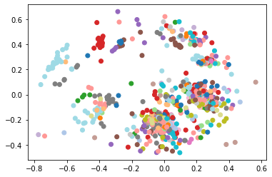 | 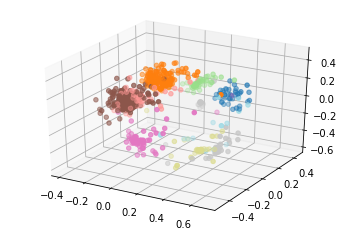 |  |
| Country of Legislator | 3d Party Scatterplot | Dot Product Networks |
Descriptions of Code and Materials
The raw data downloaded from the sources described above is contained in the Raw_Data folder, while the .csv files generated as a result of the processing procedures are contained in Processed_Data. There is one Jupyter notebook for each legislative body that does the processing and generates the relevant figures.
References
[1] Lewis, Jeffrey B., Keith Poole, Howard Rosenthal, Adam Boche, Aaron Rudkin, and Luke Sonnet (2020). Voteview: Congressional Roll-Call Votes Database. https://voteview.com/
[2] Cherepnalkoski, Darko; Karpf, Andreas; Mozetič, Igor and Grčar, Miha, 2016, Dataset of European Parliament roll-call votes and Twitter activities MEP 1.0, Slovenian language resource repository CLARIN.SI, http://hdl.handle.net/11356/1071.