This project was submitted in partial fulfillment of the Udacity Machine Learning Engineer Nanodegree.
Scott Penberthy
November 1, 2016
Self-driving cars are fascinating. However, the learning curve is steep. We noticed a lack of simple environments for experimenting with the underlying algorithms in pedagogical settings. We have built one such environment here, which a programmer can run just fine without expensive GPUs.
Our virtual environment is a derivative of Matt Harvey's virtual car, ported to work with TensorFlow, Python 2.7, and PyGame 5.0. The machine learning algorithm is based on Deep Q Reinforcement Learning, without the "deep" part. Many of the ideas were derived from songotrek's Tensorflow implementation of DeepMind's Atari-playing Deep Q Learner
Your job is to write an AI for a simulated toy car that learns to drive by itself.
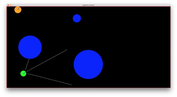
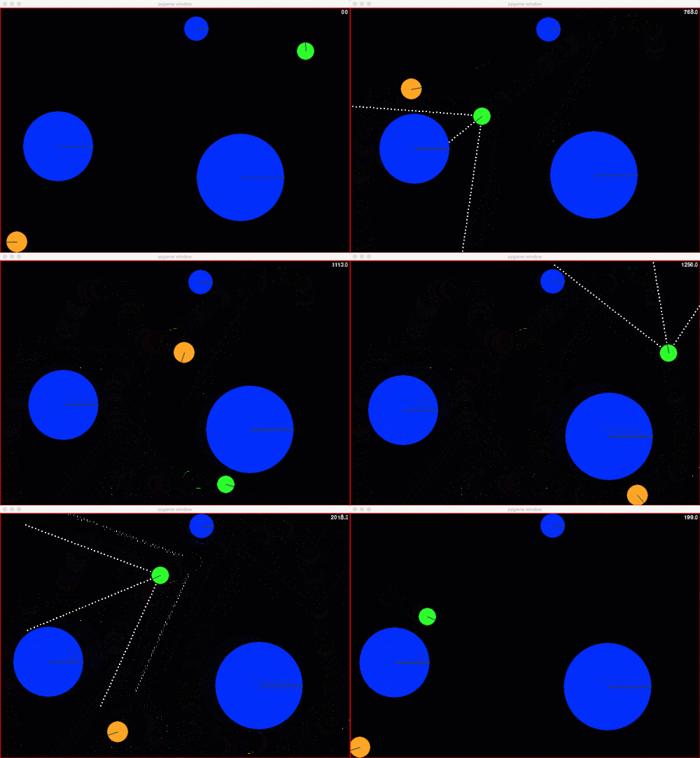
The figure above captures our toy car scenario. The car is shown in green, sensing the environment via three sonar sensors. Three slow-moving obstacles are shown in blue. A cat darts around the environment in orange. Our challenge is to build a learning algorithm that learns to drive without hitting things. The car's throttle is stuck in the "on" position. Hey, its a cheap toy.
- Anaconda Python Distribution, 2.7 for Python
- Tensorflow for Anaconda for AI
- PyGame for graphics
- PyMunk for physics
- Numpy for math
- SciPy for more math to smooth plots
This has been successfully tested on a MacBook Pro running OS X El Capitan.
After successfully cloning this repository and installing all the prerequisites, cd to
the repository directory so we have access to learning.py and carmunk.py. Let's activate
the TensorFlow environment and launch an interactive python shell:
% source activate tensorflow
(tensorflow) % ipython
Python 2.7.12 |Continuum Analytics, Inc.| (default, Jul  2 2016, 17:43:17)
Type "copyright", "credits" or "license" for more information.

IPython 5.1.0 -- An enhanced Interactive Python.
?         -> Introduction and overview of IPython's features.
%quickref -> Quick reference.
help      -> Python's own help system.
object?   -> Details about 'object', use 'object??' for extra details.

In [1]:
Next, let's import our file then create our Deep Q learner environment in one line of code!
In [1]: from learning import *

In [2]: ai = Learner()
[ed. At the time of this writing, you may see warning statements on a Mac about using outdated audio controls. That's OK. We don't need audio for this task.]
The ai object is our Deep Q Learner, without the deep, controlling a simluated game g
analyzed by a Tensorflow session s. Let's get into it. Try the following to demo 1000 steps of
the simulator and watch the car drive! At this point the algorithm is purely random.
In [3]: ai.demo()You can try each step yourself, going straight, left or right. You'll see three items returned, the reward, an array of sensor readings, and a boolean indicating whether you've hit a wall or object:
In [4]: ai.g.step(0)
(-2.0, array([ 6.        ,  4.        ,  6.        ,  0.13147931,  0.16259441,
         4.68615124]), False)

In [5]: ai.g.step(1)
(-2.0, array([ 4.        ,  4.        ,  6.        ,  0.12923619,  0.14867274,
         4.48615124]), False)


In [6]: ai.g.step(2)
(-3.0, array([ 5.        ,  3.        ,  5.        ,  0.12897384,  0.13439194,
4.68615124]), False)We will evaluate our algorithm by comparing its top score performance in 1000 games against an agent that picks actions randomly. That's all that matters in the end -- bragging rights for the most number of iterations before a crash. We need to do (much) better than random chance.
As we seek to beat random chance and improve our performance, we'll also want to track how well our algorithm is progressing. We will be tracking QMax as described in the Deep Q Learning paper.
Technically, Qmax is the maximum Q value seen by the neural network that's learning to estimate the Q function, across all training examples, across time. As the agent learns its better able to predict what action to take, leading to higher rewards over time. The longer the agent stays alive, the greater the reward, the higher the Q value.
We'll use the TensorBoard visualizer available with Tensorflow to see our top score and QMax change over time. Our learning agent sits and observes for several thousand iterations before learning. Like Mom taught us, it pays to listen and observe before making judgment!
Tensorboard runs as a local Java application, serving web pages as its GUI on a local port. This is Google, after all. The visualizer reads log data from the "train" subdirectory and periodically updates the display as log data grows. I find that periodically cleaning this directory is quite useful.
To see this work, let's mute the graphic display and run 25,000 iterations:
In [7]: ai.mute()
True

In [8]: for i in range(25000): ai.step()
Now launch another terminal and cd to the repository directory, activating tensorflow
as before. You'll see new content in the
log directory. Your log filename will be different than mine, a combo of time and your local machine
name. Launch tensorboard and point to this directory.
% source activate tensorflow

(tensorflow) % ls train
events.out.tfevents.1476194157.Scotts-MBP.home

(tensorflow) % tensorboard --logdir train
Starting TensorBoard 23 on port 6006
(You can navigate to http://0.0.0.0:6006)
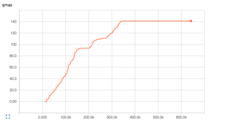
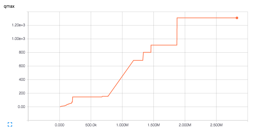
Launch your browser and navigate to http://0.0.00:6006. You'll see three numbers we're tracking, loss, qmax and score. Loss represents the amount of error in a random sample of historical frames, taken every learning cycle. QMax and Score are tracked over time, too. Click to reveal or hide plots. One example of the QMax plot is shown below, showing how are agent improves over 500k iterations. The staircase effect is caused by jumps in capability whenever the agent would copy its training network to the target, live network.
If you're curious, click on the "histograms" tab to see our network weights and biases change over time as shown below. "q_train" refers to the training network that feeds on the memory of the last 32,000 events. A "bn" metric represents the bias values with "wN" weights value in neural network that computes yN = wN*x + bN.
Here's how to read the chart.
Each vertical slice in time is a modified statistical box plot, which shows the first and second standard deviations as a band of dark (1) and lighter (2) orange, with a faded orange for outliers. When we plot these bands closely together and connect the regions, we get a flowing orange shape showing our distribution "on the side" as the statistical mean shifts over time.
The simulator provides the following information about the car at every cycle:
- s1, s2, s3 - 3 sensor readings from 0-40
- x - x position, [0,1] where 0 is far left, 1 far right
- y - y position, [0,1] where 0 is top, 1 bottom
- theta - the heading angle of the car, 0 to 2*pi
You're allowed to take three actions:
- 0, stay on course
- 1, turn left by 0.2 radians
- 2, turn right by 0.2 radians
In addition to the sensor readings, the simulator also returns the following at each iteration:
- Reward, an integer in [-100, 10] where negative values are bad, positive values are good
- Terminal, a boolean indicating whether a crash has occurred
Our challenge is to choose an action (0,1 or 2) at each time step. We're only given the state (s1,s2,s3,x,y,theta), a prior reward, and a boolean.
When we're driving free and clear, the reward varies over the interval [-4, 34] which represents the shortest distance recorded by a sonar sensor offset by -6. Thus, if one sensor has a reading of 2, the reward will be -4.
A crash occurs when a sensor reading of 1 senses an object, returning a reward of -100. The simulator randomly shifts and rotates the car in an attempt to "get free" from the obstacle. Think of this as an amygdala-driven safety reaction to danger, like a cat springing into the air at the sight of a cucumber.
The x and y position are floating point numbers varying from 0 to 1, indicating how far along each axis we sit. The angle is measured in radians, varying from 0 to 2*Pi. These measurements are a replacement for "SLAM" technology that simultaneously creates maps of the environment from richer sensor data. The hope here is that the learning algorithm figures out to stay closer to the middle, to turn away from walls, and to avoid objects when they're getting close.
Here we see an animation of the environment where actions are chosen at random. The green car moves and not that well. Each time it collides with an object, wall, or cat, the screen blinks red. The sensors are shown as white dots eminating from the car. These are the lines used to detect the distance to objects.
We can see this in slow motion, too, controlling updates with our mouse
movement and
terminating with control-C. We flip the mute switch until it returns
False, meaning that the display will be active. We call the explore
method of our learning agent. Each mouse or keyboard action
advances the play, printing out the current time step, the six
state values [s1, s2, s3, x, y, theta] and the reward R. While
the visual animation is easier to understand, the numbers
give us a sense of the actual input to the learning algorithm.
In [8]: ai.mute()
Out[8]: True

In [9]: ai.mute()
Out[9]: False

In [10]: ai.explore()
11 [0.1, 0.675, 0.375, 0.19214722317827213, 0.2243449725383465, 0.14323944878270578] R= -3.0
12 [0.075, 0.825, 0.375, 0.19979564505111702, 0.2335480823560278, 0.11140846016432673] R= -2.0
13 [0.1, 0.9, 0.675, 0.20857147067002074, 0.24039701862180216, 0.07957747154594766] R= -3.0
14 [0.075, 0.8, 0.35, 0.21621989254286564, 0.24960012843948348, 0.11140846016432673] R= -2.0
15 [0.1, 0.875, 0.7, 0.2249957181617694, 0.2564490647052578, 0.07957747154594766] R= 10.0
16 [0.575, 0.4, 0.4, 0.23454908305302546, 0.260670781943277, 0.04774648292756859] R= 6.0
^C
KeyboardInterrupt:

In [11]:
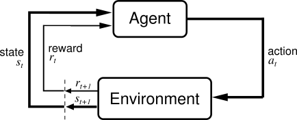
This toy car scenario can be formalized by the diagram above. We have an agent, the car, at the top of the diagram. At a point in time t we must choose an action a_t. This agent interacts with environment, causing the state of the environment s_t+1 to change in the next time step t+1. In addition the agent receives a perceived reward r_t. The agent then considers the tuple (s_t, a_t, s_t+1, r_t) and decides upon the next action a_t+1. This repeats ad nauseum.
The machine learning literature calls this a reinforcement learning problem. Each action is "reinforced" through positive or negative "reward", getting us closer or farther away from a desired "state." Let's define a function Q(s_t,a_t) as the expected, cumulative reward of taking action a_t in state s_t. How might we calculate this magical function Q?
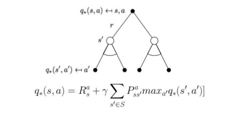
We can define this recursively as a dynamic programming problem. Q(s_t,a_t) becomes the reward r_t we receive for taking action a_t, plus the best cumulative reward available in the new state s_t+1. The best reward is then the maximum Q(s_t+1,a_t+1) available in s_t+1. The best action to take in a state is always the action a_t that has the highest Q value. This leads to the insightful, recursive Bellman equation:
Bellman defines a learning parameter, gamma, that tells us how much of our previous estimate of q(s,a) we want to believe when updating values (from 0-100% or 0.0-1.0). We want to learn slowly and deliberately, ironing out statistical outliers. Gamma is often quite close to 1.0, or 0.9 in our case.
This seems easy enough, but how do we pick initial Q values? What's interesting is that, over infinite time, it doesn't really matter! With infinite iterations of this algorithm the values of Q(s,t) will settle to an optimal plan. Common practice starts with something reasonable, namely some white Gaussian noise around 0.
Many implementations keep track of a "Q state table" which we update every cycle based on actions and observations. This is fine for simple puzzles and games, but it quickly falls apart for domains with very large state sets. The toy car example uses floating point numbers for the sensors, position and angle, and has an infinite state space.
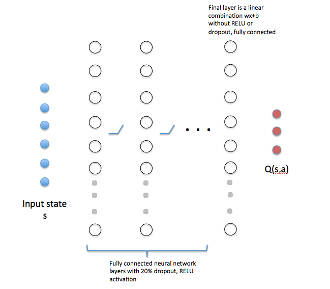
We replace the state table with a neural network shown below. We use the existing state s_t as the input values. These are then fed through multiple hidden layers with nonlinear activation and dropout, followed by a final linear combination layer. The output layer corresponds to a single neuron for each potential action, which in this case yields 3 nodes.
In our code, the number of nodes in each hidden layer are kept in an
array n_hidden. For example the code below specifies a network with a first layer of 64 neurons,
followed by 3 layers of 128 nodes each, then a final linear layer of 64 nodes:
In [10]: n_hidden =[64] + [128]*3 + [64]The neural network "learns" the Q state table by solving a non-linear regression, mapping an input state s to the numerical values for Q(s,a_i) for all actions a_i. For our scenario, we have 6 input variables and 3 output variables. Keeping in line with earlier observations about Q(s,t), we initialize the network with white noise. The weights are Gaussian noise about 0, with a standard deviation of 0.01. The biases are all positive, again at 0.01, shifting the solution space slightly away from 0.
That's fine, but how what do we "train" this network? Isn't that supervised learning, where we want the ultimate solution?
This is the ingenius trick of the Deep Q Learning crowd. They use two copies of the neural network, one to train, and another to calculate the Q(s_t+1, a_t+1) "target" values. The "training" network feeds not on the current actions, but on a sample of recent history called a "minibatch." We calculate the maximum Q(s,t) values of the minibatch, then use this as the target value when adjusting weights in the training network (via gradient descent, minimizing the squared error between our predicted Q values and the target Q values). We repeat until we've completely refreshed the recent history. At that point in time we copy all the weights from the training network to the active, target network and repeat.
The target network drives actions in the simulator and updates the recent history. We keep the training network "offline" to prevent thrashing. If you look carefully at our QMax values from before, you'll notice a staircase effect as the values climb over time. Each step up occurs when the smarter training network is copied to the target network. Neat, huh?
We want to ensure that our algorithm is doing better than random chance. We seed all the random generators to 0, then evaluate the agent by playing 1000 consecutive games. The score of a game is defined by the number of frames before a crash occurs, at which point a game ends. The car recovers like a cat jumping from a cucumber, then the next game begins. We report basic statistics on the scores from the 1000 games. The score to beat is 192.
We normalize input parameters so they all fall between 0 and 1. This prevents bias towards parameters with larger absolute values.
The x,y positions are left unchanged. The angle theta is modulated by 2 Pi, then scaled by 1/(2 Pi). In earlier versions of the code we found that the angle would increase into the thousands of radians, sending our network into a tailspin as biases would shift. The modolu fixed that. Sensor readings are scaled by 1/40.
We explored scaling the rewards similarly, between -1.0 and 1.0. This was done in the original deep Q learning paper so that various Atari games were treated similarly. Perhaps it was impatience, but we found that the network failed to learn much in the first million iterations. The higher reward values made learning easier, as the reward "signal" stood out from the Gaussian noise embedded within the network. With smaller reward values, the Gaussian noise hid the signal and the network floundered.
However, one of the rewards was confounding our efforts. The negative reward of -500 for a crash was too severe, so we scaled it back to -100 so that our reward mean was closer to 0.
Here's the problem we discovered. During backpropagation that adjusts weights in the network, we look to minimize loss. Our loss was the sum of squares between predicted Q(s,a) and target Q(s,a) values. The reward for most states falls in the 0-40 range given the maximum distance a sonar travels without hitting an object. Further, this range had a mean of 20. Our network begins with output values that are close to zero with a bit of white Gaussian noise. That means our initial loss is typically 400-1600. The network would adjust weights to reduce this number closer to 0.
Now assume we're near an optimal loss, then a crash happens, perhaps due to the cat approaching us from behind. The crash introduces a loss of 250,000, more than 100x worse that what we typically see. This spike sends a shockwave through the neural network, causing weights to take a larger step down a gradient curve to account for the error. However, this large step can have a deleterious effect on other outputs, skipping over local and global minima, pushing us much further from optimum. The network slowly recovers and starts fine-tuning the network to handle the most common case. Then, a crash happens, and we kick the network into another tail spin.
This would repeat ad-nauseum. We'd see the network approach a minimal loss, experience a spike, and the loss would swing wildly.
Mathematically speaking, our original problem space has an unusually large bias towards one parameter, creating a non-uniform shape that is difficult to traverse with gradient descent. The large bias creates significant, numerical cliffs in the gradient space. Its as though we were traversing a mountain, get near a peak, then slipped off the edge and fell into an abyss, only to slowly climb up the hill again and repeat the process. Not fun.
Reducing the magnitude of the reward lowers the bias, softens the cliffs, and makes our network less prone to these oscillations. The lesson learned here is that we need rewards to stand out from the white Gaussian noise, but irregular or dramatic shifts can wreak havoc on gradient descent. We call this reward normalization.
Our implementation consists of essentially two files.
carmunk.py is a port of the original CarMunk
car driving game so that it works properly with PyMunk 5.0 and Python 2.7.
learning.py is an implementation of Deep Q reinforcement learning using Tensorflow
for building our neural network. We say our implemenation is "without the deep," as our network
is a simple, fully-connected network versus their deep convolutional network with hundreds of layers. We
are not operating from pixels, nor do we want to insist on an expensive GPU.
We focus on a simpler, pedagogical problem of three sensors
and toy game physics.
The environment begins by loading learning.py, instantiating a Learner() object, then
invoking a few simple commands. Let's work through it.
As a good measure, cd to the directory
where you've loaded this repository, activate the virtual Tensorboard Python environment,
clean out the training log data, launch
tensorboard as a background process, and launch
an interactive Python shell. I often run tensorboard in a separate terminal window
and let it sit.
% source activate tensorflow

(tensorflow) % rm train/*

(tensorflow) % tensorboard --logdir train &
[ some logging output will appear]

(tensorflow) % ipython
Let's load and instantiate a Learner class within our iPython shell:
In(1): from learning import *

In(2): ai = Learner()
You should see a separate window with our game environment, paused at the initial state. Let's make sure everything is working. Try 1000 steps:
In(3): ai.demo()
Games played  36
Epoch Max score 95
Epoch Mean score 27.4444444444

In (4):
The demo will print out basic statistics for your score and how many games were played. Score is the frame count before a crash.
Now let's train for a bit. We have a routine "cycle" that runs 100,000 but steps 10,000 (an "epoch") at a time. This will "mute" the graphics display for speed. After every 10,000 steps, we print out our current time, then an array showing the mean "loss" encountered in our training batches, the minimum lass, the standard deviation, and the maximum loss.
In(4): ai.cycle()
t= 11000
[654.53412, 322.84866, 86.578796, 1414.0239]
Let s be the states in a minibatch whose size is specified by
n_batch_size taken from a state memory of size n_memory_size.
Loss is the difference between
the sum of squares of Q(s,a) for all actions a as calculated
by the training network, versus the desired output which is the
sum of squares of (reward_a + Max(Q(s',a))) as calculated
by the target network for action a. Recall that this is Bellman's equation, and
we want to train our network to produce a nonlinear regression so that
Q(s,a) is accurate, for all actions, in one feed forward pass.
After we have seen n_observe steps, we also print descriptive statistics
for the performance of our network every time we copy the trained network
to our target network, as specified by n_network_update_frames. Recall
that the Deep Q Learning algorithm trains a separate network on minibatches
of experience history while it simultaneously runs the agent using a
target network. This prevents thrashing and overfitting.
In(4): ai.cycle()
t= 11000
[654.53412, 322.84866, 86.578796, 1414.0239]
Games played  539
Epoch Max score 144
Epoch Mean score 30.3580705009
t= 21000
[474.16202, 251.2959, 79.489487, 1243.3118]
Games played  774
Epoch Max score 223
Epoch Mean score 42.6255319149
t= 31000
[388.32297, 202.05305, 79.290771, 1086.0581]
Games played  1020
Epoch Max score 153
Epoch Mean score 40.5081300813
t= 41000
[470.96552, 234.70471, 129.87579, 1320.3688]
Games played  1281
Epoch Max score 251
Epoch Mean score 38.3908045977
t= 51000
[549.32666, 203.20442, 176.22263, 1079.8307]
Games played  1546
Epoch Max score 226
Epoch Mean score 37.7773584906
t= 61000
[610.16583, 232.79211, 224.97626, 1264.9712]
Games played  1759
Epoch Max score 484
Epoch Mean score 46.5774647887
...
As you can see, the top score is slowly but gradually improving!
Let's talk a bit about Tensorflow, the library we use for our neural network, which will be new to many researchers.
Tensorflow has a Python front-end where you first define all the input variables, the networks, and the output variables. This forms a data pipeline, much like the graphics pipelines common in videogames. When you "run" a network forward, Tensorflow interacts with a compiled implementation in C and C++ and returns the values to Python. This scales to larger networks by running that same code in a distributed manner, where the intense computations can be run in the cloud, or soon in the cloud with hardware acceleration via TPUs and GPUs. When we "run" the backpropagation, Tensorflow performs the matrix determinants and multiplications with the C and C++ code, adjusting weights and returning values.
Tensorboard is a visualizer for variables, weights, biases and more. You'll see a rather peculiar trick, where we stuff the values for our maximum Q value and maximum Score from Python into Tensorflow on every iteration. Tensorboard can only report on values stored in the C/C++ pipeline. We dump the results to the log file every 100 iterations to keep the log file sizes in check. This took me a bit of time to figure out.
In a separate browser window, navigate to "http://0.0.0.0:6006" to see Tensorbard visualizations of our network as it trains, which we showed earlier. The repository begins with the good network which consists of 8 layers. Tensorboard will show you the weights as wN and biases as bN for each layer, as well as the loss, q_max, and top score over time.
A lot of these libraries were new for me. The primary challenges were grok'ing how to work with Tensorflow and Tensorboard, and the separation of variable space between Python and the C/C++ data pipeline. Next, PyGame and PyMunk had released a new version of the code that broke the original CarMunk, so we had to figure out both the physics library and the gaming environment. Finally, we had to implement the Deep Q Learning algorithm but substitute our simpler, pedagogical network for their convolutional network.
The longest standing bug was an improper treatment of the target and training networks. For a few weeks I was training and simulating the same network, then copying it to an offline target. Wrong. My learner kept thrashing and not progressing well, causing me to wonder if simple networks would even work! By careful digging in the related research to Deep Q Learning, I found a paper that explained how neural networks are unstable when you train and drive reinforcement learning at the same time. Well, how about that. I carefully analyzed the code and found my mistake. Once that was in place, the learners took off!
Originally I had planned to introduce a simple approach for working with GPUs, too. After blowing a few hundred dollars on GPU hosting, though, I felt that was unreasonable for an academic exercise, and switched gears to simpler networks. I also wanted to share my carefully honed Docker containers. Wrestling NVida, Amazon, Docker, Tensorflow, PyGame, and MatPlotLib proved frustrating. Even after I got them running, the cost of the daily container would exceed $500/month for 1 GPU, and one wasn't interesting. I sense market opportunity...
We started with the best network ideas available online, namely a two-layer network. This worked quite well, but we were annoyed that the car kept crashing. We tried several tricks from the literature:
- Like Deep Q, we initially stacked the last four (4) state readings into a single input. This got us to 120 for QMax.
- We increased the stacking to 16. This got us to 140 Qmax, and seeemed to be the alltime winner.
- We tried a shallow network with limited nodes (two layers of 32 nodes) and a single input. This got us nowhere, often worse performance than random. The interactions would seem random. While we could see the entire picture of what was going on, the poor agent only had three feelers. Its like feelings around in the dark with 3 poles. Our agent was often surprised by the cat or a large object from behind, or backing into a wall.
- We ran a grid search on a two-layer network, from 32 nodes to 512 nodes each. The larger networks would take longer to train. Yet, our top value for QMax wouldn't budge over 140, often ending up less. We took the best network and let it run for 2 million iterations. No joy.
- We tried a smaller memory size and larger batch size. The network would thrash, as documented in literature. We needed a much larger memory (32,000 events) with a smaller batch size of 32.
- We tried more sensors. We added sensors to the back of the car. We saw the agent learn faster, with fewer iterations. Still, the car was crashing and the 140 QMax was not exceeded. We needed a better internal representation of what was going on. Two layers wasn't cutting it.
Finally, we wondered if going deep was the answer. We created a narrow but 8-deep neural network, starting with 32 nodes, then 6 layers of 64 nodes, then a final layer of 32 nodes. This quickly got to our magical 140 and sat there for hundreds of thousands of iterations. We let it run over the weekend.
The network trained slowly, as though the intelligence was seeping in from the right. We'd see the weights and biases of the farthest networks to the right change first, then slowly affect the early networks. When those kicked in we saw a significant jump. The narrow, deeper network had blasted through and was now achieving scores in the thousands with a Qmax nearly 10x the best grid iterations. This one was a keeper.
We evaluated our final agent while it played 1000 games. The network had certainly learned to navigate the environment better than random chance. Our top score beat the random agent by an order of magnitude. The mean score across all games was over 3x better than random, but we skewed toward much higher values with a standard deviation again nearly 10x the random agent. We matched the low values, namely, where the toy car restarts and instantly crashes. This can occur from the crude approach we take for recovering from a crash, which can leave the agent close to an obstruction.
We chose a deeper, narrow network to learn the Q function that drove the simulation you see above. This was one of the trickier moves. Our final agent used the normalized sensor readings (described earlier) as the input layer. We specified our layers as follows:
In[12]: n_hidden = [32] + [64]*6 + [32]The input was fully connected to the first hidden layer of 32 artificial neurons, which was passed through a 20% dropout and then a linear rectifier (RELU). The dropout helps prevent overfitting. The output of these were fully connected to another layer of 64 neurons, and again passed through a 20% dropout and a RELU. We repeated this six (6) times. The final 64-neuron layer was fully connected to a layer of 32 neurons. These, in turn, were fully connected to the output layer of 3 neurons corresponding to the Q values for going straight (0), turning left (1), or turning right (2). We then trained this agent over 2.8 million iterations, creating the changes in QMax seen below.
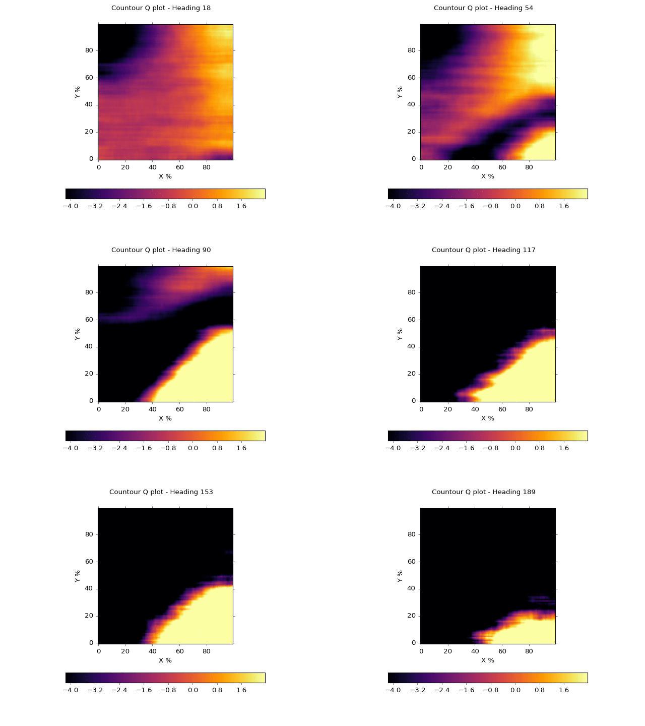
Visualizing a neural network can be challenging. The animation below is one attempt.
The x-axis represents the x location as it ranges from left (0) to right (100%). The y-axis represents the y location as it ranges from bottom (0) to top (100%). We fix the sensor readings at 20% strength each, or 0.2. We create a heat map where the darker, cooler colors represent a low Q score, and brighter, hotter colors represent a high Q score. We then animate the heatmap by rotating the toy car from facing to the right (0 degrees) to facing to the left (180 degrees) in 20 equal increments. We've smoothed out the noise to get a better sense of what the network is "thinking."
You'll note that the network believes a wide, center stripe through the diagonal is a reasonably safe area
when heading to the right. As the car rotates left from 0 to 180 degrees, however, this band narrows
and the network prefers having the
car in the lower right. This makes sense. If you're heading left, you'd like to be on the far right
and away from the left wall. This code can be seen in plotting.py.
The random movement of the cat, the slow moving objects, and the random start over thousands of games trained the agent to deal with multiple anomalies. The agent appears robust to changes in the environment.
However, the agent still crashes! We observe that this often occurs upon recovery, where the "restart" places our toy car in a precarious position with the throttle at full power. The agent also can't see behind its movement with the simple sensors. The agent often turns and collides as though the objects suddenly appeared. In fact, they have! The sensors can't tell the difference.
What's clearly missing here is an internal model of the environment. The original Deep Q Network had most of the pixels, then numerous convolution layers to analyze the world. Our agent has 3 feelers. All objects and walls look the same and we only see three pinholes around us.
This toy car needs to create an internal model for the items in its environment, their direction of movement, as well as the stationary walls. The walls form a static "map" and modeled items are "road hazards." This is the job of GPS and SLAM in self-driving cars, or Simultaneous Localization and Mapping. With a map in hand and a picture of nearby road hazards, we can more effectively plan a route and navigate through tight spaces. We also avoid being "surprised" and turning into an obstacle.
We also need better control of the car. Having the throttle on full is dangerous indeed. We need braking, stopping, starting and acceleration, as well as more nuanced control of the driving direction.
The final model achieved a peak performance that was 86.2 standard deviations greater than the peak performance of the random agent, a clear outlier. Our final model delivered a mean performance in the 95th percentile of the random agent, 3.06 standard deviations above the mean.
Our final model had a performance distribution that skewed right, with a standard deviation of 220.8 and a mean of 100. When crashes occur, they seem to occur early. This is consistent with our observation that crashes often happen in clusters upon recovery, delivering many short games. The "smarter" agent was able to keep many games going much longer, into the thousands of frames. The learning was achieved after an initial plateau. We found that, indeed, the deeper models performed better than the shallow, 2-layer models.
Our original goal of creating a simple environment for exploring autonomous vehicles in Tensorflow was achieved. We have
- created a reinforcement learning agent
- implemented a simplified version of Deep Q learning in Python and Tensorflow
- demonstrated shallow vs. deeper networks and their capability
- leveraged Tensorflow for visualization and computation
- leveraged a gaming environment for live visualization
- exposed problem areas in autonomous vehicles, seeing a need for maps, SLAM and better sensors.
I can see now why pedagogical environments are rare. Tensorflow and Deep Q Learning have a substantial learning curve. Worse, the deep convolutional networks today require expensive, custom hardware to achieve a modicum of performance. Current offerings are limited in that the latest CUDA software, Docker containers, Tensorflow libraries, Python libraries, and APIs are in flux and often incompatible. Still, we were able to build one environment that I hope others get to enjoy.
As for the toy example, several hours playing with the model cause me to scream for better sensors. The simple, "pinhole" views of our surroundings are woefully insufficient for planning and detecting collisions. Even still, watching our networks learn, experimenting with different shapes, and getting to know the Tensorflow tools was quite educational and rewarding.
An enhanced, 3D environment would be fun and more realistic, much like aerospace engineers use flight simulators. This would allow us to simulate a Lidar and more sophisticated sensors. We could also add code for creating internal models of the other agents in the 2D game based solely on sensor data. We could add better controls for the car, including braking, pausing, and accelerating, as well as a smarter crash recovery technique.
Finally, we could downscale the simulation and implement this with full pixel input, following the research of the original Deep Q Learning team. That might veer too far from the pedagogical intent.
