This package allows you to explore using the double logistic function for describing the selectivity pattern for use in length- and age-based fisheries assessment models. The double logistic function is useful because the standard logistic or sigmoidal selectivity curve is a special case of the double logistic for some parameter configurations. The double logistic can allow for dome shaped selectivity.
It is a six parameter model and therefore it is quite demanding. So for example for a catch at age model where there are 6 or less age classes for which selectivity is estimated, it is better just to estimate selectivity for each age as it is more flexible and may even use less df. I suspect this is why it is not used that much in model fitting though SS3 uses it. For length based models or when trying to catchability*selectivity correct an abundance at length survey time series, then this kind of selectivity function could be more useful. Whatever, the case it is useful to see how the parameters affect the shape of the curve.
A double logistic function can be written in several different ways. It is the product of two logistic curves and some of the parameterisations seem fairly intuitive while less so for others. The one used here is: (the latex equation does not render properly in github a markdown file so the gif of the equation is also included
Where SL is the selectivity at length, L is length, α1 is the slope of the first (ascending) logistic curve α2 is the slope of the second (descending) logistic curve, β1 is the inflection point of the first (ascending) logistic curve, β2 is the inflection point of the second (descending) logistic curve, Ω1 is the maximum selectivity level of the curve for simple logistic and Ω2 is the minumum asymptotic selectivity level of the curve.
This parameterisation contains the intuitive points that a fisheries modeller would think about when trying to develop a selectivity curve for a particular species, stock and gear type.
The inflection points are the points of maximum steepness of each of the selectivity curves, i.e. the minimum length of fish where the majority are caught by the gear. The slopes describe how much selectivity changes for a unit change in size, i.e. how quickly (in terms of fish length) a gear goes from low to high selectivity for individuals. The first slope describes the initial increase in selectivity while the second describes the descending part of the curve if it is dome shaped. The slopes and inflections together tend to describe the width of the plateau in selectivity of a dome shaped curve. The final parameter is the asymptotic selectivity level for a dome shaped curve. If you want just a simple logistic curve you can set Ω2=Ω1.
library(devtools)
install_github("duplisea/dublogistic")
Load the package
library(dublogistic)
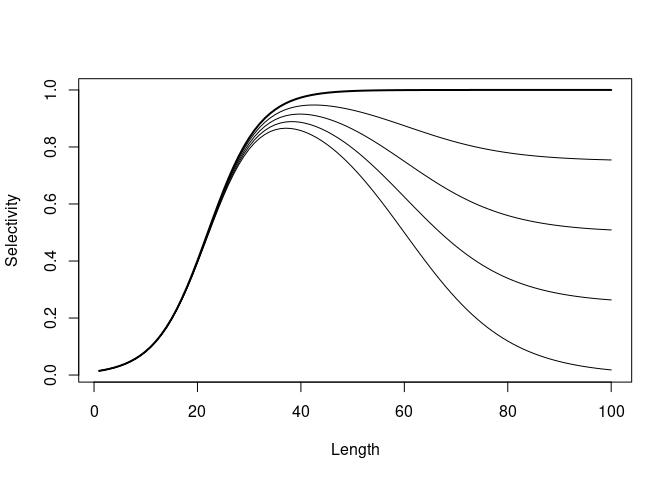
We start with the doming aspect of the double logistic because it is likely the reason you would be considering it. This is done by changing the parameter minsel.upper (miniumum selectivity of the upper part of the curve).
L= 1:100
sel= dublogistic.f(L=L, inflection1=22, inflection2=60, slope1=0.2, slope2=0.1, max.sel=1, minsel.upper=1, plot=T)
lines(dublogistic.f(L=L, inflection1=22, inflection2=60, slope1=0.2, slope2=0.1, max.sel=1, minsel.upper=0.75, plot=F))
lines(dublogistic.f(L=L, inflection1=22, inflection2=60, slope1=0.2, slope2=0.1, max.sel=1, minsel.upper=0.5, plot=F))
lines(dublogistic.f(L=L, inflection1=22, inflection2=60, slope1=0.2, slope2=0.1, max.sel=1, minsel.upper=0.25, plot=F))
lines(dublogistic.f(L=L, inflection1=22, inflection2=60, slope1=0.2, slope2=0.1, max.sel=1, minsel.upper=0, plot=F))
You can see that by changing the asmyptotic selectivity for large sizes, it also changes the maximum selectivity lelvel of the curve even though that max is set equal to 1. You may need to play around with it. There is possibly an analytic formulation which preserve the maximum parameter as a function of the asymptotic selectivity value. Just eye-balling it, it looks like square root or perhaps just a ratio.
L= 1:100
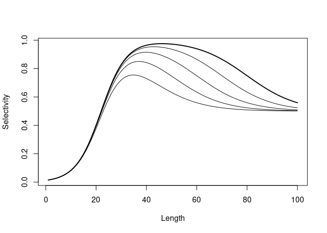
sel= dublogistic.f(L=L, inflection1=22, inflection2=80, slope1=0.2, slope2=0.1, max.sel=1, minsel.upper=0.5, plot=T)
lines(dublogistic.f(L=L, inflection1=22, inflection2=50, slope1=0.2, slope2=0.1, max.sel=1, minsel.upper=0.5, plot=F))
lines(dublogistic.f(L=L, inflection1=22, inflection2=60, slope1=0.2, slope2=0.1, max.sel=1, minsel.upper=0.5, plot=F))
lines(dublogistic.f(L=L, inflection1=22, inflection2=70, slope1=0.2, slope2=0.1, max.sel=1, minsel.upper=0.5, plot=F))
lines(dublogistic.f(L=L, inflection1=22, inflection2=40, slope1=0.2, slope2=0.1, max.sel=1, minsel.upper=0.5, plot=F))
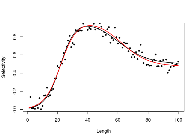
The black line is the real curve and the red the fitted line. It is really difficult to fit in reality so starting values matter a lot. The example only adds a small amount of noise and it can be interesting to explore how well it fits with more noise (try it). I found that when the sd of the normal noise is 0.25 or greater, nls cannot converge.
L=1:100
sel= dublogistic.f(L=L, inflection1=22, inflection2=60, slope1=0.2, slope2=0.1, max.sel=1, minsel.upper=0.5, plot=T)
fit.data=sel
fit.data$selectivity= fit.data$selectivity+rnorm(length(fit.data$selectivity),0,.05)
names(fit.data)= c("L","sel")
points(fit.data, pch=20)
dl.formula= as.formula(sel~(max.sel/(1+exp(-slope1*(L-inflection1))))*(1-minsel.upper/(1+exp(-slope2*(L-inflection2)))))
dl.fit= nls(dl.formula,data= fit.data, start=list(inflection1=20, inflection2=70, slope1=.3, slope2=.05, max.sel=1, minsel.upper=.5))
lines(fit.data$L,predict(dl.fit),col="red",lwd=2)
You can also fit a double logistic using the sicegar library which has a more sophisticated approach to fitting the model and also distinguishes if a dataset is best fit with a logistic or double logistic. Apparently, it is a common problem in cell and bacterial growth modelling in medical sciences.
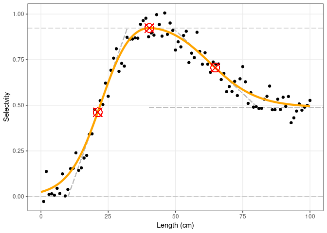
So let’s fit it with sicegar (I copied these code lines from the sicegar vignette). This makes a pretty ggplot graph and it also fits the data properly. The sicegar model fits a different parameterisation of the model though and I have not gone through to see how those parameters relate to one used above.
library(sicegar)

dataInput= data.frame(time=fit.data$L,intensity=fit.data$sel)
fitObj <- fitAndCategorize(dataInput,threshold_minimum_for_intensity_maximum = 0.3,threshold_intensity_range = 0.1, threshold_t0_max_int = 0.05)

sicegar.fit <- figureModelCurves(dataInput = fitObj$normalizedInput,doubleSigmoidalFitVector= fitObj$doubleSigmoidalModel, showParameterRelatedLines = TRUE)
sicegar.fit$labels$y="Selectvity"
sicegar.fit$labels$x="Length (cm)"
plot(sicegar.fit)
Caglar et al. (2018), Sicegar: R package for sigmoidal and double-sigmoidal curve fitting. PeerJ 6:e4251; DOI 10.7717/peerj.4251


