flexplot

Overview

flexplot is a set of tools designed to pair with statistical modeling and simplify the process of visualizing data analysis. Some of the primary functions include:

flexplot() flexible and intelligent multivariate graphics
added.plot() added variable plots
visualize() shows a visual representation of a fitted object
compare.fits() visually compares the fit of two different models
estimates() reports of effect sizes for statistical models
model.comparison() statistically compares the fits of two different models

A more complete manual for flexplot can be found at the Psych Arxiv

Installation of flexplot

# install.packages("devtools")
# install the stable version
devtools::install_github("dustinfife/flexplot")
# install the development version
devtools::install_github("dustinfife/flexplot", ref="development")

Usage

library(flexplot)
data(relationship_satisfaction)

### multivariate relationship
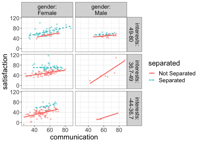
flexplot(satisfaction~communication + separated | gender + interests, data=relationship_satisfaction)

### show a straight line, remove standard errors, and specify 3 bins
flexplot(satisfaction~communication + separated | gender + interests, data=relationship_satisfaction, method="lm", se=F, bins=3)

### show a ghost line to simplify comparisons
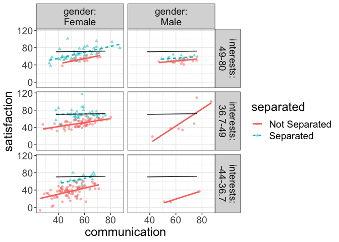
flexplot(satisfaction~communication + separated | gender + interests, data=relationship_satisfaction, method="lm", se=F, bins=3, ghost.line="black")

### categorical variable
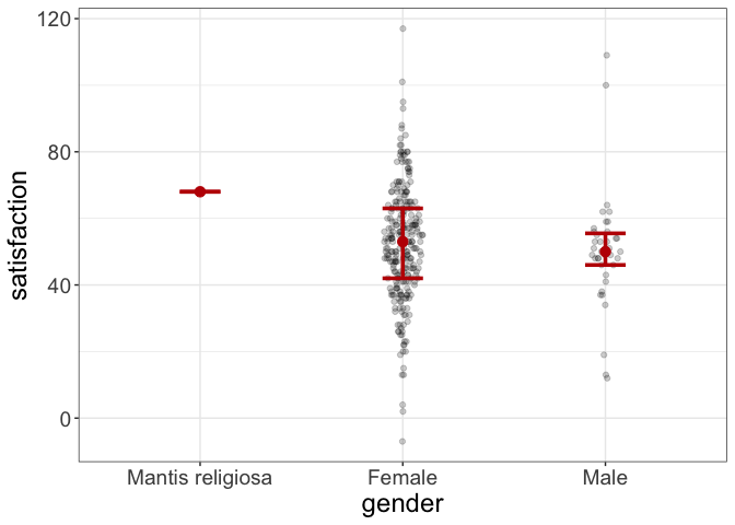
flexplot(satisfaction~gender, data=relationship_satisfaction, spread="quartiles", jitter=c(.1, 0))

### histogram/barchart
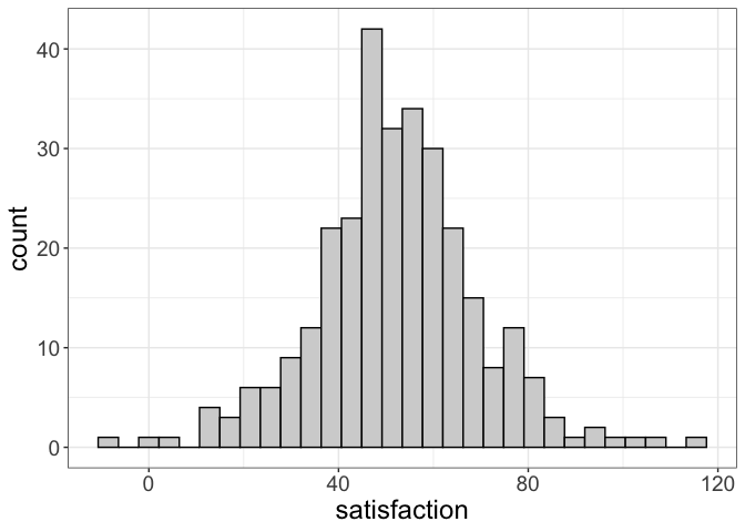
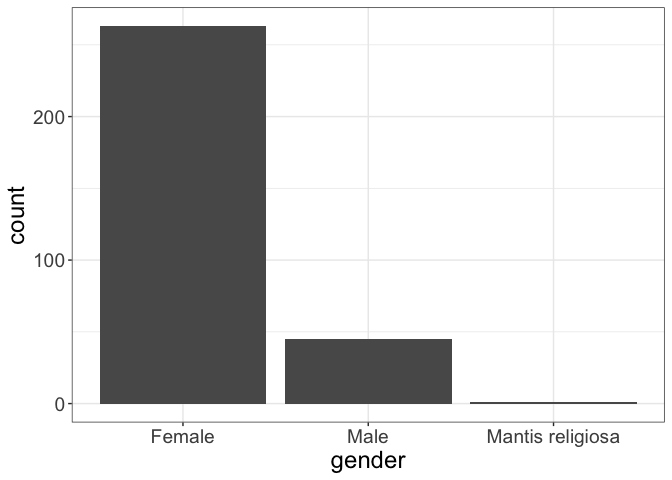
flexplot(satisfaction~1, data=relationship_satisfaction)

flexplot(gender~1, data=relationship_satisfaction)

### added variable plot
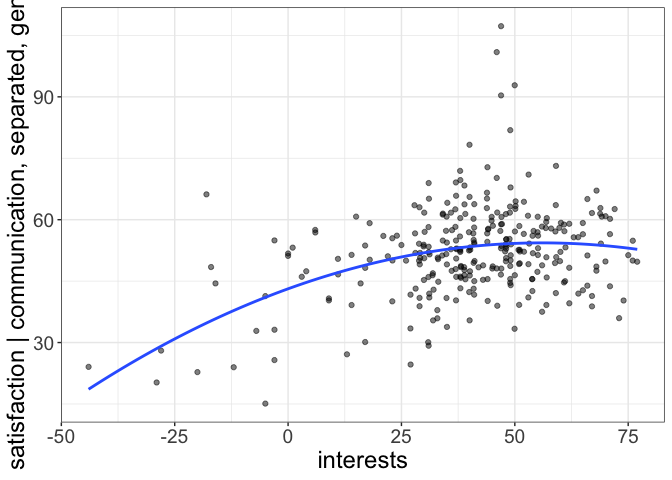
added.plot(satisfaction~communication + separated | gender + interests, data=relationship_satisfaction, method="polynomial", se=F)

### modeling + graphics
full.mod = lm(satisfaction~communication * separated , data=relationship_satisfaction)
reduced.mod = lm(satisfaction~communication + separated , data=relationship_satisfaction)
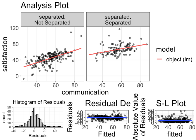
visualize(full.mod)

estimates(full.mod)
#> Model R squared:
#> 0.567 (0.49, 0.64)
#> 
#> Semi-Partial R squared:
#> communication:separated 
#>                    0.01 
#> 
#> Estimates for Factors:
#>   variables        levels estimate lower upper
#> 1 separated Not Separated    44.72  43.1 46.35
#> 2               Separated    65.78 63.56    68
#> 
#> 
#> Mean Differences:
#>   variables              comparison difference lower upper cohens.d
#> 1 separated Separated-Not Separated      21.06  17.2 24.91     1.84
#> 
#> 
#> Estimates for Numeric Variables = 
#>       variables estimate lower upper std.estimate std.lower std.upper
#> 1   (Intercept)     2.66 -5.28 10.59         0.00      0.00      0.00
#> 2 communication     0.76  0.62  0.91         0.49     -0.47      1.45
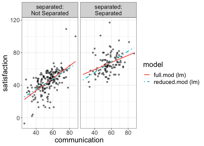
compare.fits(satisfaction~communication|separated, data=relationship_satisfaction, full.mod, reduced.mod)

model.comparison(full.mod, reduced.mod)
#> $statistics
#>                  aic      bic bayes.factor p.value r.squared
#> full.mod    2312.712 2331.214        1.566  0.0108     0.567
#> reduced.mod 2317.309 2332.111        0.639             0.557
#> 
#> $pred.difference
#>    0%   25%   50%   75%  100% 
#> 0.033 0.460 0.962 1.814 6.736

Getting help

If something breaks, please post a minimal reproducible example on github. For questions and other discussion, contact me on twitter or by email.