WHAT IS DATA SCIENCE?

Data Science is about data gathering, analysis and decision-making. It is about finding patterns in data, through analysis, and make future predictions.

By using Data Science, companies are able to make:

Better decisions (should we choose A or B)
Predictive analysis (what will happen next?)
Pattern discoveries (find pattern, or maybe hidden information in the data.

How does Data Scientist Work?

A Data Scientist requires expertise in several backgrounds:

Machine Learning
Statistics
Programming (Python or R)
Mathematics
Databases A Data Scientist must find patterns within the data. Before he/she can find the patterns, he/she must organize the data in a standard format.
Here is how a Data Scientist works:

Ask the right questions - To understand the business problem.
Explore and collect data - From database, web logs, customer feedback, etc.
Extract the data - Transform the data to a standardized format.
Clean the data - Remove erroneous values from the data.
Find and replace missing values - Check for missing values and replace them with a suitable value (e.g. an average value).
Normalize data - Scale the values in a practical range (e.g. 140 cm is smaller than 1.8 m. However, the number 140 is larger than 1.8 - so scaling is important).
Analyze data, find patterns and make future predictions.
Represent the result - Present the result with useful insights in a way the "company" can understand.

PYTHON LIBRARIES

Python is a widely used programming language by Data Scientists. In this course, we will use the following Python libraries:

Pandas
Numpy
Matplotlib
SciPy

Create your Virtual Environment, etc.
Install Pandas pip install pandas

PANDAS

pandasintro.py

Pandas is an open source python library providing high performance data manipulation and analysis tool using its powerful data structures. Pandas involve 2 structures:

Series - a single dimension with a homogenous data type values. series()
DataFrame - a two dimension data structure with heterogenous data type elements. pd.DataFrame()

Import the Pandas library as pd
Define data with column and rows in a variable named d
Create a data frame using the function pd.DataFrame() -- (note the Capital D and F)
The data frame contains 3 columns and 5 rows
Print the data frame output with the print() function

Advantages of Pandas:

Easy handling of missing data
Data can be sliced, merged, concatenated and reshaped. Before analyzing data, a Data Scientist must extract the data, and make it clean and valuable.

EXTRACT DATA

extracting_data.py

Pandas is a library in Python used for data analysis and data manipulation. To import data, we us read_csv() function to import CSV file.

Import the Pandas library
Name the data frame as health_data.
header=0 means that the headers for the variable names are to be found in the first row (note that 0 means the first row in Python)
sep="," means that "," is used as the separator between the values. This is because we are using the file type .csv (comma separated values)

POINTS TO NOTE:

Blank rows - data set loaded using Pandas automatically converts blank cells to NaN
dropna() function can be used to remove NaNs

health_data.dropna(axis=0,inplace=True)
print(health_data)

axis=0 means that we want to remove all rows that have a NaN value

DATA CATEGORIES

Data can be split into three main categories:

Numerical - Contains numerical values. Can be divided into two categories:
- Discrete: Numbers are counted as "whole". Example: You cannot have trained 2.5 sessions, it is either 2 or 3
- Continuous: Numbers can be of infinite precision. For example, you can sleep for 7 hours, 30 minutes and 20 seconds, or 7.533 hours
Categorical - Contains values that cannot be measured up against each other. Example: A color or a type of training
Ordinal - Contains categorical data that can be measured up against each other. Example: School grades where A is better than B and so on

ANALYSE DATA

We can use describe() function in Python to summarize data

Count - Counts the number of observations
Mean - The average value
Std - Standard deviation (explained in the statistics chapter)
Min - The lowest value
25%, 50% and 75% are percentiles (explained in the statistics)
Max - The highest value

MATHS

Mathematical functions are important to know as a data scientist, because we want to make predictions and interpret them.

LINEAR FUNCTIONS

Here, a function is used to relate one variable to another variable.

A linear function has one independent variable (x) and one dependent variable (y).

If we consider the relationship between calorie burnage and average pulse. It is reasonable to assume that, in general, the calorie burnage will change as the average pulse changes - we say that the calorie burnage depends upon the average pulse.

Furthermore, it may be reasonable to assume that as the average pulse increases, so will the calorie burnage. Calorie burnage and average pulse are the two variables being considered.

Because the calorie burnage depends upon the average pulse, we say that calorie burnage is the dependent variable and the average pulse is the independent variable.

y = f(x) = ax + b

This function is used to calculate a value for the dependent variable when we choose a value for the independent variable.

Explanation:

f(x) = the output (the dependant variable)
x = the input (the independant variable)
a = slope = is the coefficient of the independent variable. It gives the rate of change of the dependent variable
b = intercept = is the value of the dependent variable when x = 0. It is also the point where the diagonal line crosses the vertical axis.

Linear Function With One Explanatory Variable

A function with one explanatory variable means that we use one variable for prediction.

Let us say we want to predict calorie burnage using average pulse. We have the following formula:

f(x) = 2x + 80

Here, the numbers and variables means:

f(x) = The output. This number is where we get the predicted value of Calorie_Burnage
x = The input, which is Average_Pulse
2 = Slope = Specifies how much Calorie_Burnage increases if Average_Pulse increases by one. It tells us how "steep" the diagonal line is
80 = Intercept = A fixed value. It is the value of the dependent variable when x = 0

PLOTTING LINEAR FUNCTION

Linear means "straight line".

In plotting a graph, key factors:

Horizontal axis is the X axis
Vertical Axis is the Y axis

MATPLOTLIB

This is a plotting library. we will plot the values of Average_Pulse against Calorie_Burnage using the matplotlib library. The plot() function is used to make a 2D hexagonal binning plot of points x,y

matplotlibintro.py

Example Explained:

Import the pyplot module of the matplotlib library
Plot the data from Average_Pulse against Calorie_Burnage
kind='line' tells us which type of plot we want. Here, we want to have a straight line
plt.ylim() and plt.xlim() tells us what value we want the axis to start on. Here, we want the axis to begin from zero
plt.show() shows us the output

The picture(graph) explained:

There is a relationship between Average_Pulse and Calorie_Burnage. Calorie_Burnage increases proportionally with Average_Pulse. It means that we can use Average_Pulse to predict Calorie_Burnage.
The reason the line doesn't start from 0, 80 is the first observation of Average_Pulse and 240 is the first observation of Calorie_Burnage.
As it turns out:
- If the average pulse is 80, the calorie burnage is 240
- If the average pulse is 90, the calorie burnage is 260
- If the average pulse is 100, the calorie burnage is 280

There is a pattern. If average pulse increases by 10, the calorie burnage increases by 20.

SLOPE AND INTERCEPT:

slope_and_intercept.py

f(x) = 2x + 80

we'll explain how the figure for the function y = f(x) = ax + b was gotten.

Find the Slope:

The slope is defined as how much calorie burnage increases, if average pulse increases by one. It tells us how "steep" the diagonal line is.

We can find the slope by using the proportional difference of two points from the graph:

If the average pulse is 80, the calorie burnage is 240
If the average pulse is 90, the calorie burnage is 260

We see that if average pulse increases with 10, the calorie burnage increases by 20.

Slope = 20/10 = 2

The slope is 2.

Mathematically, the calculation for slope is defined as: slope = fx2 - fx1 / x2 - x1

fx2 = Second observation of Calorie_Burnage = 260
fx1 = First observation of Calorie_Burnage = 240
x2 = Second observation of Average_Pulse = 90
x1 = First observation of Average_Pulse = 80

Slope = (260-240) / (90 - 80) = 2

Find the Intercept:

The intercept is where the diagonal line crosses the y-axis, if it were fully drawn. In other words, it is the intercept is the value of y, when x = 0.

In our health data, we can see that when average_pulse (x) is 0, Calorie_Burnage (y) is 80. Thus, the intercept is 80. Sometimes, the intercept has a practical meaning, other times it doesn't. However, we need to include the intercept in order to complete the mathematical function's ability to predict Calorie_Burnage correctly.

Other examples where the intercept of a mathematical function can have a practical meaning:

Predicting next years revenue by using marketing expenditure (How much revenue will we have next year, if marketing expenditure is zero?). It is likely to assume that a company will still have some revenue even though if it does not spend money on marketing.
Fuel usage with speed (How much fuel do we use if speed is equal to 0 mph?). A car that uses gasoline will still use fuel when it is idle.

Finding the Slope and Intercept Using Python

The numpy.polyfit() function returns the slope and intercept.

Explained:

Isolate the variables Average_Pulse (x) and Calorie_Burnage (y) from health_data.
Call the np.polyfit() function.
The last parameter of the function specifies the degree of the function, which in this case is "1".

health_data = pd.read_csv("health_data.csv", header=0, sep=",")

x = health_data[" Average_Pulse"]
y = health_data[" Calorie_Burnage"]

slope_intercept = np.polyfit(x,y,1)
print(slope_intercept)

prints [2. 80.]

This calculates the slope and intercept; slope is 2 and intercept is 80.

Therefore, using f(x) or y = 2x + 80 if we want to calculate the Calorie_Burnage(y) when Average_Pulse(x) is 135, it is calculated f(135) = 2(135) + 80 = 350

It is written in python as:

def calculate(x):
    solution = (2 * x) + 80
    return int(solution)

print(calculate(135))
print(calculate(125)) # to clarify with the available data.

STATISTICS

Statistics is a science of analyzing data. This helps ascertain the prediction's reliability. i.e whether or not we can rely on the prediction made

statisticsintro.py

DESCRIPTIVE STATISTICS

Descriptive statistics summarizes important features of a data set such as:

Count
Sum
Standard Deviation
Percentile
Average etc

The describe() function earlier explained to summarise the data

The percentiles are used in statistics to give you a number that describes the value that a given percent of the values are lower than.

Explaning the 25% and 75% using the Average_Pulse:

The 25% percentile of Average_Pulse means that 25% of all of the training sessions have an average pulse of 100 beats per minute or lower.
The 75% percentile of Average_Pulse means that 75% of all the training session have an average pulse of 111 or lower.

To find percentile, we use numpy.percentile().

STATISTICS STANDARD DEVIATION

Standard deviation is a number that describes how spread out the observations are. It is represented as std.

Standard deviation is a measure of uncertainty. A low standard deviation means that most of the numbers are close to the mean (average) value. A high standard deviation means that the values are spread out over a wider range.

Standard Deviation is often represented by the symbol Sigma: σ Numpy has a Standard deviation function as std()

COEFFICIENT OF VARIATION

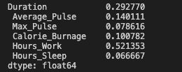
This is used to get an idea of how large the standard deviation is. It is defined mathematically as coefficient of variation = Standard Deviation (std) / Mean

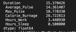
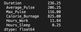
We see that the variables: Duration, Calorie_Burnage and Hours_Work has a high Standard Deviation compared to Max_Pulse, Average_Pulse and Hours_Sleep.

VARIANCE

Another way to indicate how spread the values are, is to use Variance.

Also, if you take the square root of the variance, you get the standard deviation. Or the other way around, if you multiply the standard deviation by itself, you get the variance!

Variance is often represented by the symbol Sigma Square: σ^2

How to calculate variance(using Average_Pulse):

Step 1 to Calculate the Variance: Find the Mean. We want to find the variance of Average_Pulse.

Find the mean:

(80+85+90+95+100+105+110+115+120+125) / 10 = 102.5 The mean is 102.5.

Step 2: For Each Value - Find the Difference From the Mean

Find the difference from the mean for each value:

e.g 80 - 102.5 = -22.5

Step 3: For Each Difference - Find the Square Value

Find the square value for each difference:

e.g (-22.5)^2 = 506.25

Note: We must square the values to get the total spread.

Step 4: The Variance is the Average Number of These Squared Values

Sum the squared values and find the average:

(506.25 + 306.25 + 156.25 + 56.25 + 6.25 + 6.25 + 56.25 + 156.25 + 306.25 + 506.25) / 10 = 206.25 The variance is 206.25.

To verify the result, numpy has a function var() for calculating variance or the function I wrote to find variance

CORRELATION

Correlation measures the relationship between two variables.

Earlier we said that a function has a purpose to predict a value, by converting input (x) to output (f(x)). We can say also say that a function uses the relationship between two variables for prediction.

The correlation coefficient can never be less than -1 or higher than 1:

1 = there is a perfect linear relationship between the variables (like Average_Pulse against Calorie_Burnage)
0 = there is no linear relationship between the variables
-1 = there is a perfect negative linear relationship between the variables (e.g. Less hours worked, leads to higher calorie burnage during a training session)

Example of a Perfect Linear Relationship

Correlation Coefficient = 1

We will use scatterplot to visualize the relationship between Average_Pulse and Calorie_Burnage. Thus, change kind to "scatter": correlation_stats.py

CORRELATION MATRIX

We can use the corr() function in Python to create a correlation matrix. We also use the round() function to round the output to two decimals

SEABORN

Seaborn is a visualization library based on matplotlib. It is an advance statistical and graphical representation library. We can use the Seaborn library to create a correlation heat map. Heatmap is used to Visualize the Correlation Between Variables:

pip install seaborn
Import seaborn as sn
Use the health_data set.
Use sn.heatmap() to tell Python that we want a heatmap to visualize the correlation matrix.
Use the correlation matrix. Define the maximal and minimal values of the heatmap. Define that 0 is the center.
Define the colors with sns.diverging_palette. n=500 means that we want 500 types of color in the same color palette.
square = True means that we want to see squares.

CORRELATION VS. CAUSALITY

Correlation measure the numerical relationship between two variables. Using a beach example, the sale of ice cream increases during the summer, the same for drowning accidents. However, does that mean the increase of ice cream sale is the direct cause of increased drowning accidents? corrvscaus.py

From the example, can we use the ice cream sale to predict drowning accidents? - Maybe Not; except the effects of taking too much ice cream and having side effects e.g eating before swimming etc.

However, wwhat causes drowning?

Unskilled swimmers
Waves
Cramp
Seizure disorders
Lack of supervision
Alcohol (mis)use etc.

Let us reverse the argument:

Does a low correlation coefficient (close to zero) mean that change in x does not affect y?

Back to the question:

Can we conclude that Average_Pulse does not affect Calorie_Burnage because of a low correlation coefficient?

The answer is no.

There is an important difference between correlation and causality:

Correlation is a number that measures how closely the data are related
Causality is the conclusion that x causes y.

ebosetalee/path-to-data-science