FixedPointFinder - A Tensorflow toolbox for finding fixed points and linearized dynamics in recurrent neural networks
Finds and analyzes the fixed points of recurrent neural networks that have been built using Tensorflow. The approach follows that outlined in Sussillo and Barak (2013), "Opening the Black Box: Low-Dimensional Dynamics in High-Dimensional Recurrent Neural Networks", Neural Computation.
Written using Python 2.7.12.
If you are using FixedPointFinder in research to be published, please cite our accompanying paper in your publication:
Golub and Sussillo (2018), "FixedPointFinder: A Tensorflow toolbox for identifying and characterizing fixed points in recurrent neural networks," Journal of Open Source Software, 3(31), 1003, https://doi.org/10.21105/joss.01003 .
-
Clone or download this repository.
-
Create a virtual environment for the required dependencies: To create a new virtual environment specific to Python 2.7, enter at the command line:
$ virtualenv --system-site-packages -p python2.7 your-virtual-env-name
where
your-virtual-env-nameis a path to the the virtual environment you would like to create (e.g.:/home/fpf). Then activate your new virtual environment:$ source your-virtual-env-name/bin/activateWhen you are finished working in your virtual environment (not now), enter:
$ deactivate
-
Automatically assemble all dependencies using
pipand therequirements*.txtfiles. This step will depend on whether you require Tensorflow with GPU support.For GPU-enabled TensorFlow, use:
$ pip install -r requirements-gpu.txt
For CPU-only TensorFlow, use:
$ pip install -r requirements-cpu.txt
Advanced Python users and those wishing to develop contributions may prefer a custom install. Such installs should adhere to the following general template:
-
Clone or download this repository.
-
Install compatible versions of the following prerequisites.
- TensorFlow (requires at least version 1.10) (install).
- NumPy, SciPy, Matplotlib (install SciPy stack, contains all of them).
- Scikit-learn (install).
- PyYaml (install).
- RecurrentWhisperer (install).
-
Add the directories for
FixedPointFinderandRecurrentWhispererto your Python path:$ export PYTHONPATH=$PYTHONPATH:/path/to/your/directory/fixed-point-finder/ $ export PYTHONPATH=$PYTHONPATH:/path/to/your/directory/recurrent-whisperer/
where "/path/to/your/directory" is replaced with the path to the corresponding repository. This step must be performed each time you launch a new terminal to work with
FixedPointFinder, and thus you may want to add the lines above to a startup script (e.g., the .bashrc / .bashprofile script in your home folder or an activate script in your virtual environment).
FixedPointFinder includes a test suite for confirming successful installation, and for ensuring that contributions have not introduced bugs into the main control flow. The tests run FixedPointFinder over a set of RNNs where ground truth fixed points have been previously identified, numerically confirmed, and saved for comparison.
To run the tests, descend into the test directory: fixed-point-finder/test/ and execute:
>>> python run_test.py-
Start by building, and if desired, training an RNN.
FixedPointFinderworks with any arbitrary RNN that conforms to Tensorflow'sRNNCellAPI. -
Build a
FixedPointFinderobject:>>> fpf = FixedPointFinder(your_rnn_cell, tf_session, **hyperparams)
using
your_rnn_cell, theRNNCellthat specifies the single-timestep transitions in your RNN,tf_session, the Tensorflow session in which your model has been instantiated, andhyperparams, a python dict of optional hyperparameters for the fixed-point optimizations. -
Specify the
initial_statesfrom which you'd like to initialize the local optimizations implemented byFixedPointFinder. These data should conform to shape and type expected byyour_rnn_cell. For Tensorflow'sBasicRNNCell, this would mean an(n, n_states)numpy array, wherenis the number of initializations andn_statesis the dimensionality of the RNN state (i.e., the number of hidden units). For Tensorflow'sLSTMCell,initial_statesshould be anLSTMStateTuplecontaining one(n, nstates)numpy array specifying the initializations of the hidden states and another(n, nstates)numpy array specifying the cell states. -
Specify the
inputsunder which you'd like to study your RNN. Currently, To study the RNN given a set of static inputs,inputsshould be a numpy array with shape(1, n_inputs)wheren_inputsis an int specifying the depth of the inputs expected byyour_rnn_cell. Alternatively, you can search for fixed points under different inputs by specifying a potentially different input for each initial states by makinginputsa(n, n_inputs)numpy array. -
Run the local optimizations that find the fixed points:
>>> fps = fpf.find_fixed_points(initial_states, inputs)
The fixed points identified, the Jacobian of your RNN state transition function at those points, and some metadata corresponding to the optimizations will be returned in the
FixedPointsobject.fps(see FixedPoints.py for more detail). -
Finally, visualize the identified fixed points:
>>> fps.plot()
You can also visualize these fixed points amongst state trajectories from your RNN (see
plotin FixedPoints.py and the example in run_FlipFlop.py)
FixedPointFinder includes an end-to-end example that trains a Tensorflow RNN to solve a task and then identifies and visualizes the fixed points of the trained RNN. To run the example, descend into the example directory: fixed-point-finder/example/ and execute:
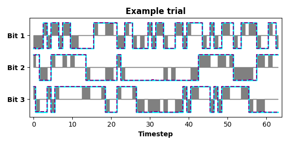
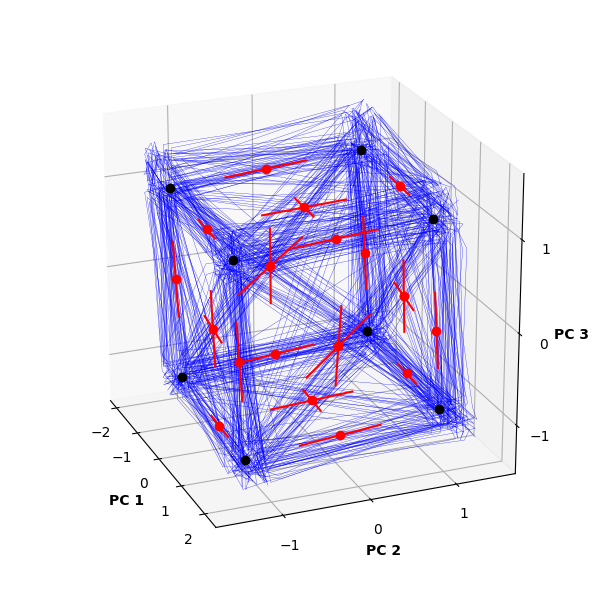
>>> python run_FlipFlop.pyThe task is the "flip-flop" task previously described in Sussillo and Barak (2013). Briefly, the task is to implement a 3-bit binary memory, in which each of 3 input channels delivers signed transient pulses (-1 or +1) to a corresponding bit of the memory, and an input pulse flips the state of that memory bit (also -1 or +1) whenever a pulse's sign is opposite of the current state of the bit. The example trains a 16-unit LSTM RNN to solve this task (Fig. 1). Once the RNN is trained, the example uses FixedPointFinder to identify and characterize the trained RNN's fixed points. Finally, the example produces a visualization of these results (Fig. 2). In addition to demonstrating a working use of FixedPointFinder, this example provides a testbed for experimenting with different RNN architectures (e.g., numbers of recurrent units, LSTMs vs. GRUs vs. vanilla RNNs) and characterizing how these lower-level model design choices manifest in the higher-level dynamical implementation used to solve a task.
Figure 1. Inputs (gray), target outputs (cyan), and outputs of a trained LSTM RNN (purple) from an example trial of the flip-flop task. Signed input pulses (gray) flip the corresponding bit's state (green) whenever an input pulse has the opposite sign of the current bit state (e.g., if gray goes high when green is low). The RNN has been trained to nearly perfectly reproduce the target memory state (purple closely overlaps cyan).
Figure 2. Fixed-point structure of an LSTM RNN trained to solve the flip-flop task. FixedPointFinder identified 8 stable fixed points (black points), each of which corresponds to a unique state of the 3-bit memory. FixedPointFinder also identified a number of unstable fixed points (red points) along with their unstable modes (red lines), which mediate the set of state transitions trained into the RNN's dynamics. Here, each unstable fixed point is a "saddle" in the RNN's dynamical flow field, and the corresponding unstable modes indicate the directions that nearby states are repelled from the fixed point. State trajectories from example trials (blue) traverse about these fixed points. All quantities are visualized in the 3-dimensional space determined by the top 3 principal components computed across 128 example trials.
Contributions are welcome. Please see the contribution guidelines.

