This project uses deep learning, specifically long-short term memory (LSTM) units, gated recurrent units (GRU), and convolutional neural networks (CNN) to label comments as toxic, severely toxic, hateful, insulting, obscene, and/or threatening. Each of the models here reaches over 98.4% accuracy on cross-validation and the held-out test set.
By improving automated detection of such comments, we can make online spaces more fruitful and welcoming forums for discussion.
These instructions will allow you to run this project on your local machine.
You can find the pre-trained word vectors below (note that if you download word vectors with fewer dimensions, you will have to change embed_size in the code):
Place these in a filepath/data directory. Create a /models directory for saved models and /preds for saved predictions on a held-out test set.
Once you have a virtual environment in Python, you can simply install necessary packages with: pip install requirements.txt
Note that if you have a GPU, you will also need to install CUDA 9.0. If you don't have a GPU, you should install Tensorflow instead of Tensorflow-GPU.
git clone https://github.com/edwisdom/toxic-comments
Either run a model individually with Python (e.g. python lstm.py) or run each of them sequentially with:
sh ./seq.sh
This section covers some of my basic research in deep learning concepts that helped me understand and implement these models.
Recurrent neural networks (RNNs) have been shown to produce astonishing results in text generation, sentiment classification, and even part-of-speech tagging, despite their seemingly simple architecture. RNNs are more powerful than regular/vanilla neural networks because they combine an input vector with a hidden state vector before outputting a vector, allowing us to encode the sequence of inputs over time that the network has already seen -- for our NLP application, this will be a sequence of words (encoded as vectors), though you can see an example with a sequence of characters below.
. This diagram shows the activations in the forward pass when the RNN is fed the characters 'hell' as input. The output layer contains confidences the RNN assigns for the next character (vocabulary is h,e,l,o); We want the green numbers to be high and red numbers to be low.")
For more on RNNs, read:
- The Unreasonable Effectiveness of RNNs
- A Beginner's Guide to RNNs
- Comparative Study of CNN and RNN for NLP
In this paper from 2015, the authors find that adding a convolutional layer to an RNN outperforms CNNs and RNNs alone for text classification tasks. The authors argue that while the recurrent part captures long-distance connections between the data (e.g. the beginning and end of sentence), the convolutional part captures phrase-level patterns. By adding a max-pooling layer afterward, a CNN can identify the most important words or phrases.
Although the authors don't include any discussion of a stacked CNN (with both small and large window sizes in order to capture both short- and long-distance patterns), other researchers have similarly found RCNNs to be more accurate for a number of classification tasks:
The data here consists of over 150,000 sentences from Wikipedia's talk page comments. The comments have been labeled by human moderators as toxic, severely toxic, obscene, hateful, insulting, and/or threatening. For more information about how the dataset was collected, see the original paper.
Note that there are a lot more "clean" comments (marked as 0 for all 6 classes of toxicity) than there are toxic. Moreover, "toxic" is by far the most common label. These class imbalances mean that we should be wary of methods like logistic regression, which would favor the majority class. Since we want to detect toxic online comments, misclassifying most comments as clean would defeat the purpose, even though it might improve model accuracy. Read here for more on the class imbalance problem.

As the following table shows, there is significant overlap between "toxic" and the other classes. For example, the sentences labeled "severely toxic" are a subset of those labeled "toxic."
| severe_toxic | obscene | threat | insult | identity_hate | ||||||
|---|---|---|---|---|---|---|---|---|---|---|
| 0 | 1 | 0 | 1 | 0 | 1 | 0 | 1 | 0 | 1 | |
| toxic | ||||||||||
| 0 | 144277 | 0 | 143754 | 523 | 144248 | 29 | 143744 | 533 | 144174 | 103 |
| 1 | 13699 | 1595 | 7368 | 7926 | 14845 | 449 | 7950 | 7344 | 13992 | 1302 |
Here, I will outline some of the major model parameters that I iteratively tweaked, along with the effect on the model's accuracy rate.
I began with a simple model:
- Embedding layer with an input of pre-trained 50-dimensional vectors (GloVe 6B.50D)
- Bidirectional LSTM of size 50, with dropout 0.1
- Pooling layer (average + max concatenated)
- FC layer of size 25, with dropout 0.1
- Output FC layer of size 6 (one per class)
I used a batch size of 32 and the Adam optimizer, which is an alternative to stochastic gradient descent. Each parameter of the network has a separate learning rate, which are continually adapted as the network learns. For more on the Adam optimizer, read here.
Keras Output:
loss: 0.0447 - acc: 0.9832 - val_loss: 0.0472 - val_acc: 0.9824
The model had trained for 2 epochs. This output from Keras shows loss and accuracy on the training data used, and the 10% held out for cross-validation. Since the out-of-sample predictions best indicate how well the model generalizes, the val_loss and val_acc will be the measures that I report for future model iterations.
First, I recognized that I could train for multiple epochs. The network eventually overfits if we add too many epochs, so first, we can add a callback to stop early. In this code, if val_loss doesn't improve after 3 epochs, the model stops training.
es = EarlyStopping(monitor='val_loss',
                   min_delta=0,
                   patience=3,
                   verbose=0, mode='auto')
Moreover, we can save the best model with the following callback:
best_model = 'models/model_filename.h5'
checkpoint = ModelCheckpoint(best_model,
                             monitor='val_loss',
                             verbose=0,
                             save_best_only=True, mode='auto')
model.fit(X_t, y, batch_size=batch_size, epochs=epochs, callbacks=[es, checkpoint], validation_split=0.1)
Second, I migrated the network to my GPU by downloading CUDA and Tensorflow-GPU. This allowed me to change the batch size to 1024 and train my network much faster.
Loss: 0.0454, Accuracy: 0.9832
I wanted to check if I could tune the model's performance by increasing dropout before experimenting with the network's architecture. Almost all of these efforts, done alone, actually lowered the model accuracy.
- Embedding Layer Dropout to 0.2 -- Loss: 0.0469, Accuracy: 0.9827
- Final Layer Dropout to 0.3 -- Loss: 0.0482, Accuracy: 0.9831
- LSTM Dropout to 0.3 -- Loss: 0.0473, Accuracy: 0.9827
- Recurrent Dropout to 0.3 -- Loss: 0.0465, Accuracy: 0.9831
These results make some sense in hindsight, since the network size is relatively small. As this paper found, applying dropout in the middle and after LSTM layers tends to worsen performance. This, of course, didn't explain why increasing dropout in the embedding layer (which comes before the LSTM) worsened performance.
As I found in this paper on CNNs, dropping random weights doesn't actually help when there is spatial correlation in the feature maps. Since natural language also exhibits spatial/sequential correlation, spatial dropout would be a much better choice, since it drops out entire feature maps. After adding a spatial dropout of 0.2 before the LSTM layer, the network finally improved.
Loss: 0.0452, Accuracy: 0.9834
First, I experimented with a different RNN cell. I simply reconstructed the previous network's architecture, but replaced LSTM cells with GRU cells. GRU layers only have two gates, a reset and update gate -- whereas the update gate encodes the previous inputs ("memory"), the reset gate combines the input with this memory.
Whereas the LSTM can capture long-distance connections due to its hidden state, this may not be necessary for identifying toxicity, since a comment is likely to be toxic throughout. For more on the difference between GRUs and LSTMs, read here. For an evaluation of the two on NLP tasks, see this paper.
Surprisingly, the GRU performed comparably to the LSTM without any further tuning.
Loss: 0.0450, Accuracy: 0.9832
Second, I used larger pre-trained embedding vectors (from 50 dimensions to 300). Furthermore, I increased the number of words that the model was using for each comment in increments of 50, going up from 100 originally to 300 once model performance stopped improving. This simple change improved performance significantly for the LSTM.
Loss: 0.0432, Accuracy: 0.09838
Third, and perhaps most importantly, I added a convolutional layer of size 64, with a window size of 3, in between the recurrent and FC layers for both the LSTM and GRU network. Although I found RCNNs rather late in my model iteration process, I've explained them above in the Background Research section.
LSTM - Loss: 0.0412, Accuracy: 0.9842
GRU - Loss: 0.0414, Accuracy: 0.9842
Finally, I decided to stack another convolutional layer of size 64, with window size 6, before the FC layer for both networks. I also tried to add a FC layer of size 64 before the output layer. Both of these slightly improved the model, although the GRU benefitted more from the additional convolution, whereas the LSTM benefitted more from the added FC layer.
| Loss By Model | CNN Layer | FC Layer |
|---|---|---|
| GRU | 0.0406 | 0.0408 |
| LSTM | 0.0411 | 0.0402 |
Ensembled together, the two best-performing networks here reach 98.48% accuracy.
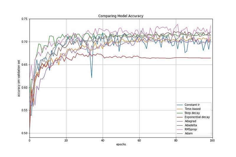
- Learning Rate Optimizers: For my data and model, Adam vastly outperformed both Adadelta, Adagrad, and RMSProp. I include a more thorough comparison of the optimizers below, from Suki Lau on Towards Data Science.
- Alternative Embeddings: All the figures I present here use the GloVe vectors, but I also tried to use pre-trained FastText vectors of the same size (300D), and the network performed comparably.
Here are some things that I did not get to tune that would make for interesting results:
- Using only max-pooling layers vs. using only average-pooling layers vs. using both
- Initializing different learning rates and setting a decay rate
- Different activation functions -- Tanh vs. PreLu vs. ReLu
- More convolutional layers with larger window sizes to capture long-distance connections
- Preprocessing comments using NLP techniques such as lemmatization, removing stop words, etc.
I would like to thank Prof. Liping Liu, Daniel Dinjian, and Nathan Watts for thinking through problems with me and helping me learn the relevant technologies faster.
I got the data for this model from a Kaggle competition, and I was helped greatly by this exploratory data analysis by Jagan Gupta.