Implementation of principal component analysis on the two-dimensional
torus
Get the latest version from GitHub:
# Install the package
library(devtools)
install_github("egarpor/ridgetorus")

# Load package
library(ridgetorus)The main functionality of ridgetorus is the function ridge_pca(),
which can be employed to do dimension reduction via the bivariate sine
von Mises (Singh et al., 2002) and the bivariate wrapped Cauchy (Kato
and Pewsey, 2015) models, as the following examples show.
# 1. Simulate data from r_bvm()
data <- r_bvm(n = 1000, mu = c(1, 2), kappa = c(5, 2, 1.5))

# 2. Do ridge_pca()
rpca <- ridge_pca(x = data, type = "bvm")

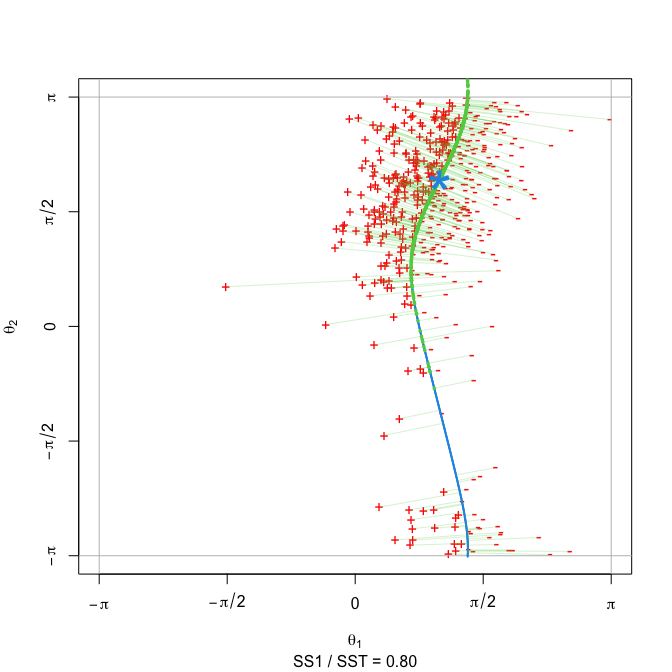
# 3. Plot simulated data with ridge fit using show_ridge_pca()
show_ridge_pca(rpca, col_data = "red")
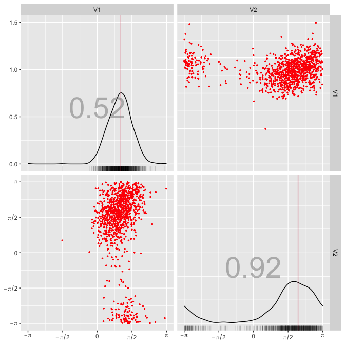
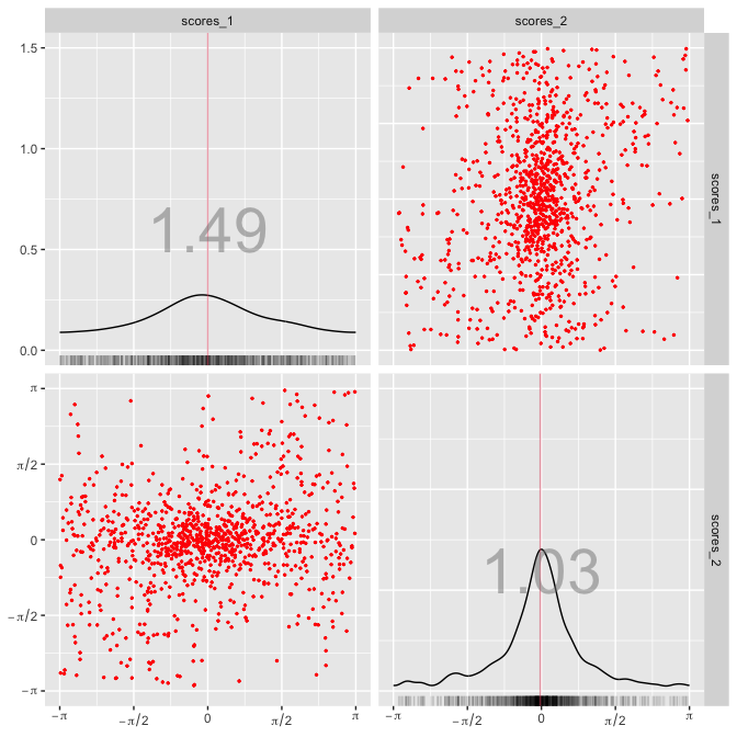
# 4. Plot pairs plots of original data and scores with torus_pairs()
torus_pairs(data, col_data = "red", bwd = "EMI")torus_pairs(rpca$scores, col_data = "red", bwd = "EMI", scales = rpca$scales)# 1. Simulate data from r_bwc()
data <- r_bwc(n = 1000, mu = c(-1, 2), xi = c(0.3, 0.6, 0.25))
# 2. Do ridge_pca()
rpca <- ridge_pca(x = data, type = "bwc")
# 3. Plot simulated data with ridge fit using show_ridge_pca()
show_ridge_pca(rpca, col_data = "red")# 4. Plot pairs plots of original data and scores with torus_pairs()
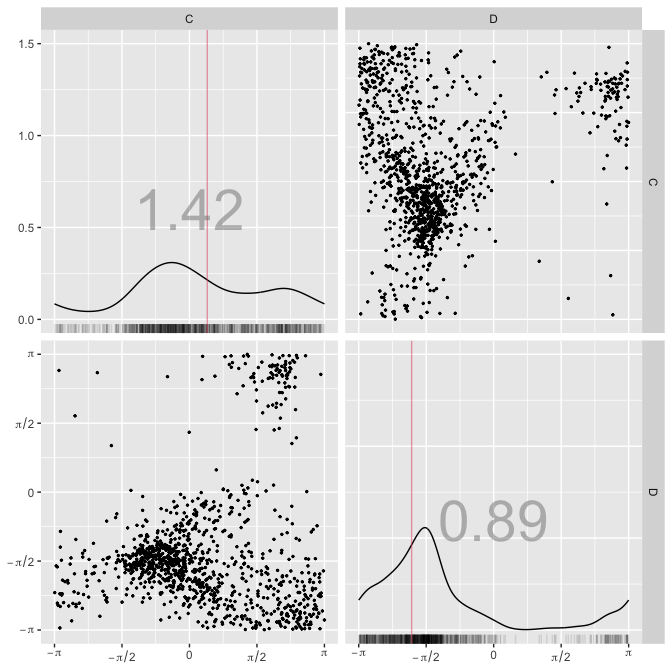
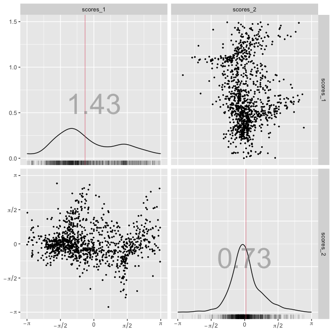
torus_pairs(rpca$scores, col_data = "red", bwd = "EMI", scales = rpca$scales)The data applications in García-Portugués and Prieto-Tirado (2023) can be reproduced through the script data-application.R. The code snippet below illustrates the toroidal PCA analysis onto currents of four zones at Santa Barbara strait. Zone A and B are on the northern coast of Santa Barbara Channel while zone C and D, are at the top and bottom ends of the interisland channel.
# Load data
data("santabarbara")

# Example with zone A-B with automatic comparison between bvm and bwc
rpca_AB <- ridge_pca(x = santabarbara[c("A", "B")], type = "auto")
show_ridge_pca(fit = rpca_AB, col_data = "black", n_max = 1e3)torus_pairs(santabarbara[c("A", "B")], col_data = "black")torus_pairs(rpca_AB$scores, col_data = "black", scales = rpca_AB$scales)rpca_AB$type
#> [1] "bwc"
rpca_AB$var_exp
#> [1] 0.7450665 1.0000000
# Example with zone C-D with automatic comparison between bvm and bwc
rpca_CD <- ridge_pca(x = santabarbara[c("C", "D")], type = "auto")
show_ridge_pca(fit = rpca_CD, col_data = "black", n_max = 1e3)torus_pairs(santabarbara[c("C", "D")], col_data = "black")torus_pairs(rpca_CD$scores, col_data = "black", scales = rpca_CD$scales)rpca_CD$type
#> [1] "bvm"
rpca_CD$var_exp
#> [1] 0.7934003 1.0000000It can be seen how the bivariate von Mises and the bivariate wrapped Cauchy are the most adequate fits for zones C–D and A–B, respectively. Toroidal PCA explains around 75% of the total variance in both cases, motivating its use for dimension reduction. The scores also transform the data distribution, reducing noise and allowing to check for groups or outliers, if any.
García-Portugués, E. and Prieto-Tirado, A. (2023). Toroidal PCA via density ridges. Statistics and Computing, 33(5):107. doi:10.1007/s11222-023-10273-9.
Kato, S. and Pewsey, A. (2015). A Möbius transformation-induced distribution on the torus. Biometrika, 102(2):359–370. doi:10.1093/biomet/asv003.
Singh, H., Hnizdo, V., and Demchuk, E. (2002). Probabilistic model for two dependent circular variables. Biometrika, 89(3):719–723. doi:10.1093/biomet/89.3.719.

