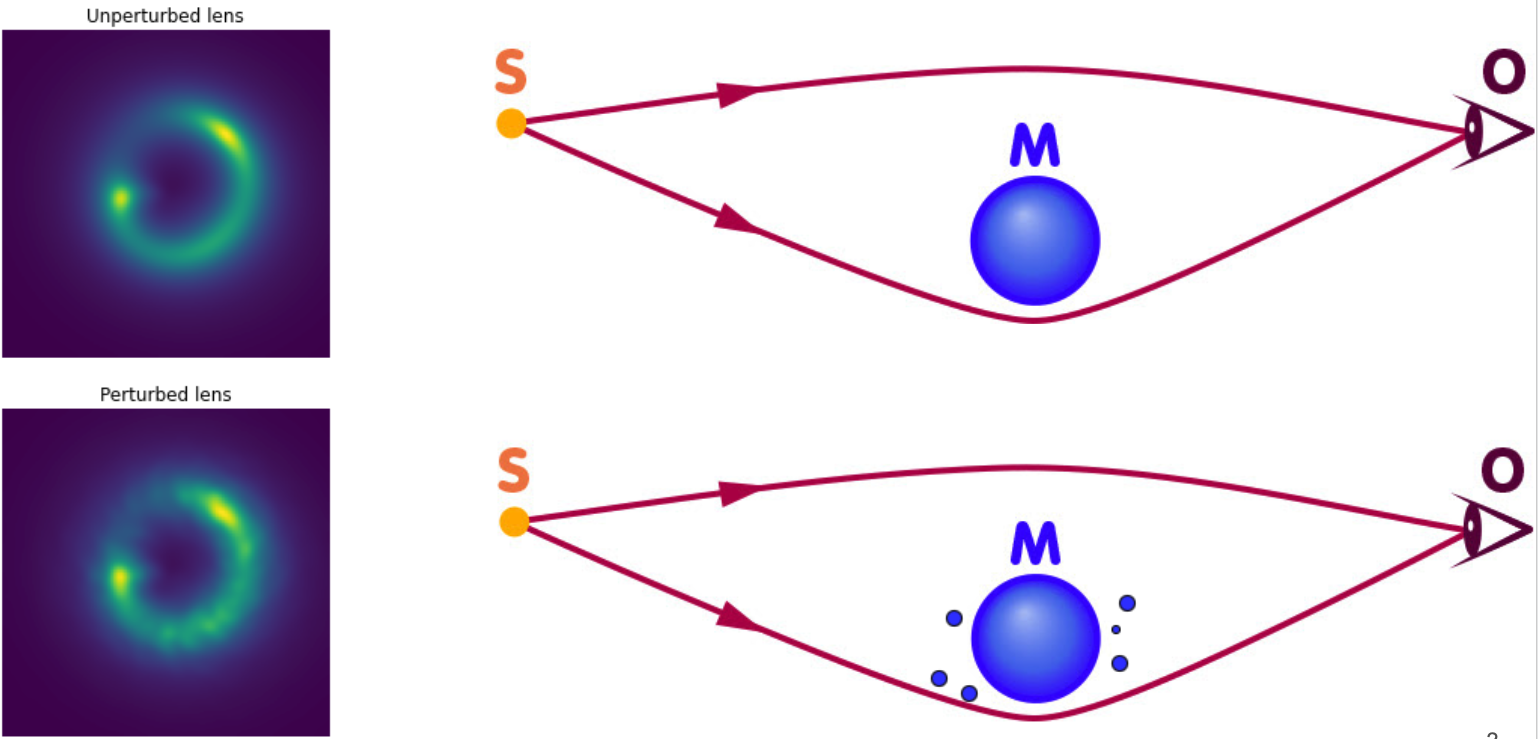
LCDM cosmological model predicts more galaxy satellites that we observe. One of the ways to find the missed satellites (if they exist) is rather than relying on an object's radiation, to use a physical effect that is determined by the object's mass. Such an effect is gravitational lensing. The amount of light deflection depends on column density along the line of sight, therefore the effect provides one with an opportunity to detect dark matter haloes, that make up most of the mass, but do not interact with light at all.
The upper row shows the classical lensing setup Source-Lens-Observer on the right and the image that the observer detects on the left. There can be not only lensing galaxy M on the line of sight, but additional mass overdensities like galaxy satellites. In this case, the total lensing potential is different from the lensing setup in the top row, hence the detected image is also different.
In this particular work, we consider additional mass that acts as a perturbation to the potential of the original lens M potential. The lower row shows exactly that case Source-Lens-Perturbations-Observer. As we want to describe the potential field with maximal simplicity, the best way is to describe the Amplitude of the field and scale of perturbation. For that case, the most useful field is a Gaussian Random Field. You can also reason the choice of a Gaussian from Central Limit Theorem. For example, if we consider many small dark matter haloes around the lens, by treating them as many random variables we can expect that their cumulative potential will be close to the normal distribution.
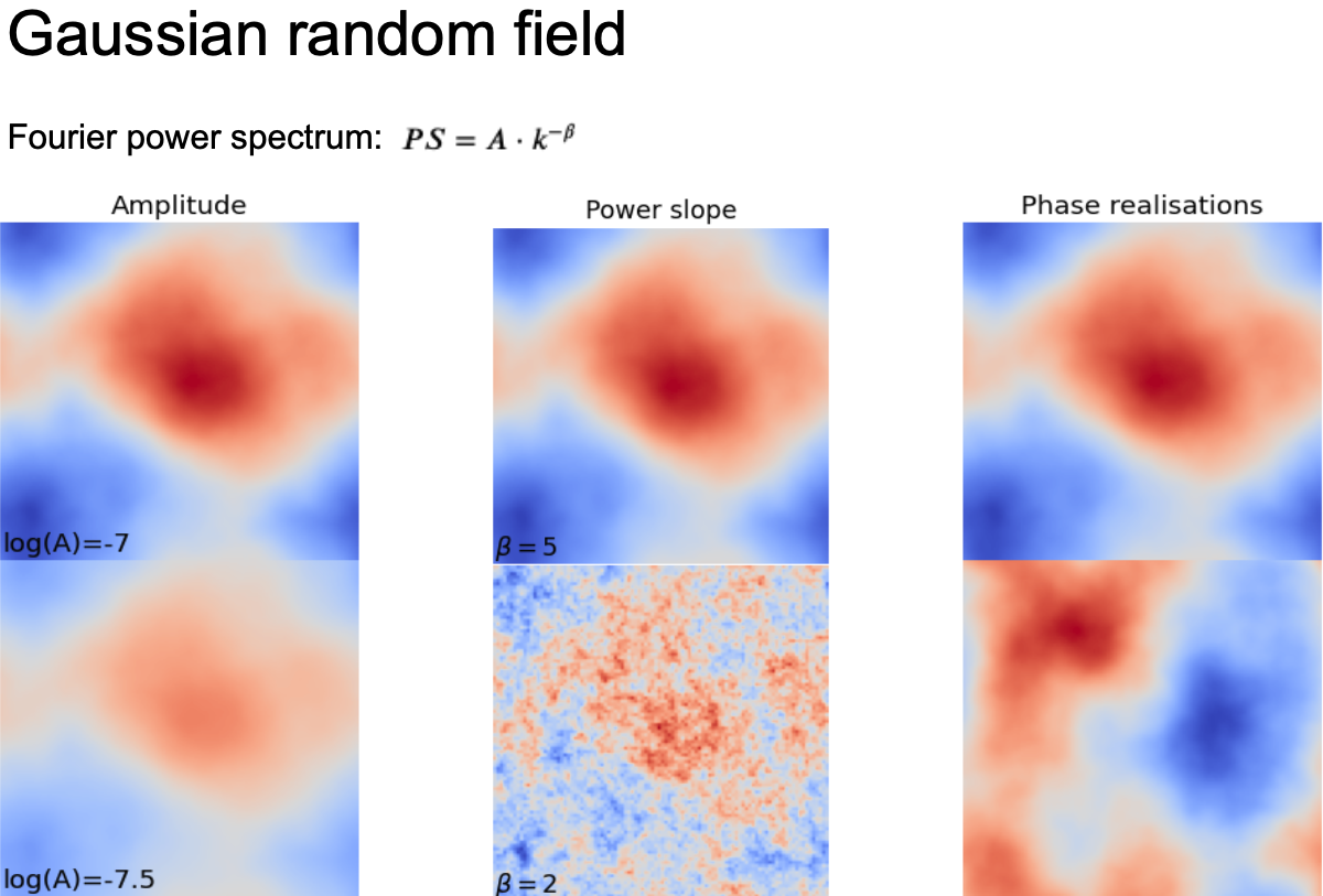
Gaussian Random Field (GRF) is defined in the Fourier space by the Power-law spectrum and Phase realization. For our simulation purposes it can be completely defined by three parameters: Amplitude “A” of the Power Spectrum PS (top of the slide), Power slope “β” and a Random seed defining the Phase realization. On the slide, you can see the separate impact of each of the variables.
The explanation for Power slope “β” is “The higher the Beta, the more power at low frequencies. The more power at low frequencies, the greater the size of the perturbations.” So “Big beta means big scale perturbations”. On the middle figure, we got a big scale blob for Beta=5 and a small scale net for Beta=2.
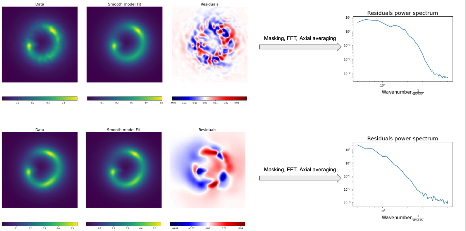
Let’s say that we have a perturbed lens image “Data”. We expect that the lens can be split into two parts: the smooth part like SIE+Shear, and the perturbation modeled by GRF. The core idea is that if we fit the “Data” using the model with only the smooth lens part, then the residuals will reflect the unaccounted perturbation lens part. One can spot a quasi-linear approach here, specifically, the fact that the perturbations are weak enough for “Data Image”≅” Smooth lensing Image”+” Perturbation lensing image”.
In the study, we want to find the power spectrum of the GRF and since the fit residuals should somehow reflect the GRF it makes sense to work with their Power Spectra.
So we mask out everything in the residuals apart of the Einstein ring region, compute the power spectrum of the masked residuals, and get axially averaged power spectrum. Working with axially averaged spectrum is reasoned by the fact that we are interested in the Amplitude of the GRF, represented by the amplitude of the Residuals Power spectrum, and in the Power Slope of the GRF, represented by the shape of the Residuals Power spectrum.
At the same time, the axial distribution of the power spectrum encodes the phase realization of the GRF, which is of no interest to us.
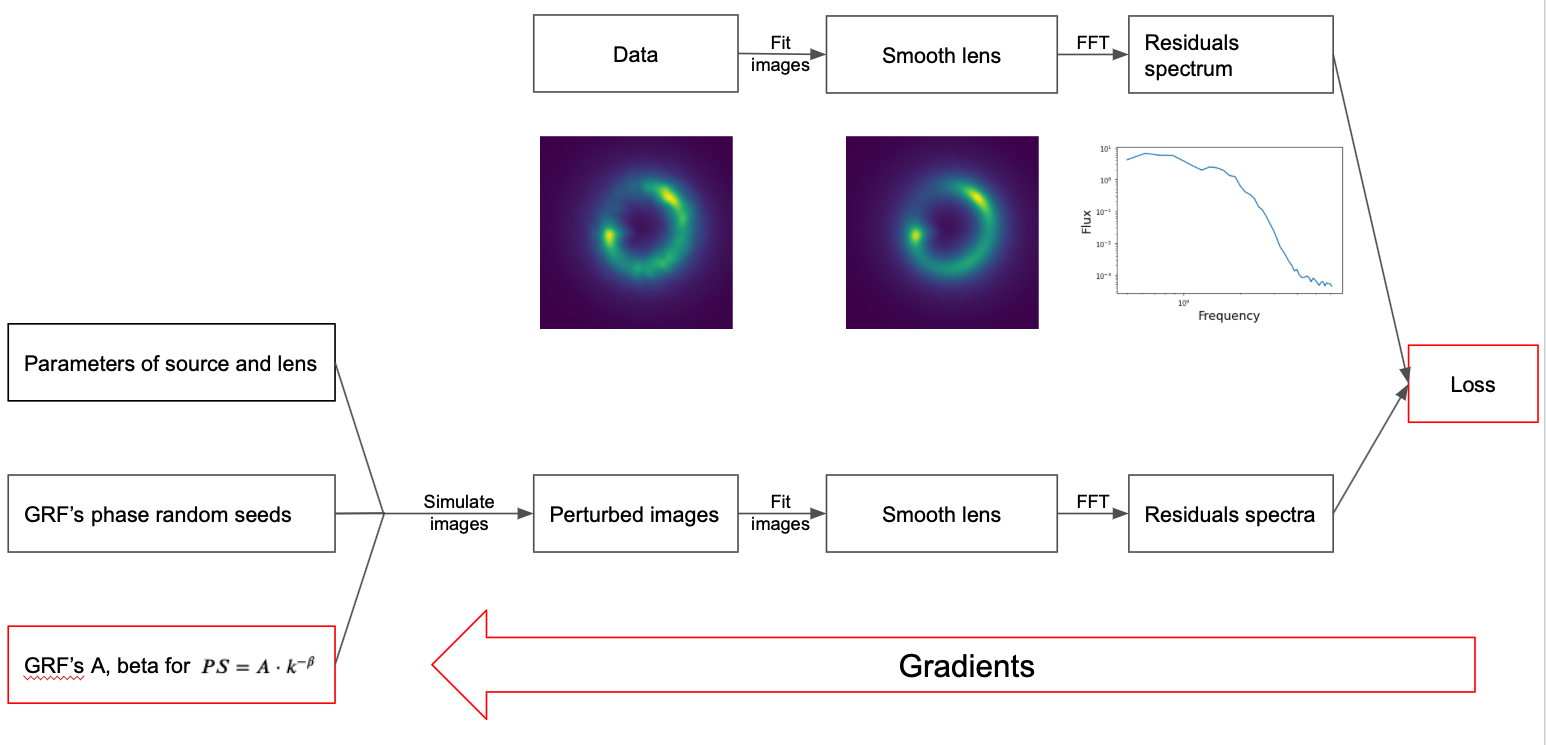
Basically, that’s the idea of the pipeline.
Out of the true source and the lens potential 𝜓0+δ𝜓 (smooth lens+GRF), nature created the “Data” image. We get the fit of the data image with smooth lens model (so get smooth potential 𝜓1) and from residuals obtain “Data power spectrum” or “PS_data”.
Then, using 𝜓1 as an approximation of 𝜓0 and GRF with controlled parameters we simulate a new perturbed lens image, fit it to get 𝜓2, and from residuals obtain “Simulation power spectrum” or “PS_simulation”.
After all, we compute the Loss function between “Data power spectrum” and “Simulation power spectrum” and estimate how close the simulated GRF is to the true one.
On the top of the figure: We can see the pipeline of obtaining the power spectrum for an observed "Data" image. In order to get the “Data power spectrum,” we fit the data, get residuals, mask them and compute axially averaged power spectrum.
At bottom of the figure: Our goal is to exactly replicate the pipeline of obtaining the “Data power spectrum”, but with controlled GRF’s Amplitude and Power slope, so we can optimize these parameters.
First step: Simulate “perturbed images” for all the GRF phase seeds. We use a smooth lens model obtained from “Data” fitting, some “GRF phase seeds” for the loss averaging, and GRF parameters A, Beta that we want to optimize.
Second step: Fit all the simulated images and compute the residuals power spectra. The tricky part is that we will need to fit each of the simulated images. Operation of fit is basically gradient descent and it should be carried out for every phase realization. Therefore the asymptotical complexity of the algorithm is O(phase number)*O(fit iterations). Fit iterations are 200, as it is the number of iterations that is usually enough for the fitted smooth model to converge. In the case of MAE, we can use phase number=1 to decrease computational complexity by the price of method accuracy. It is a way to converge from the state of absence of the GRF to the vicinity of true GRF parameters. Only then we can use more phases to converge to the true GRF parameters.
Third step: Compute Loss as an average of the distance from “Data power spectrum” to each of the “Simulated power spectra”. Given the Loss function, we can compute its gradients and hessian with respect to GRF’s A, Beta and optimize these parameters with usual optimization algorithms.
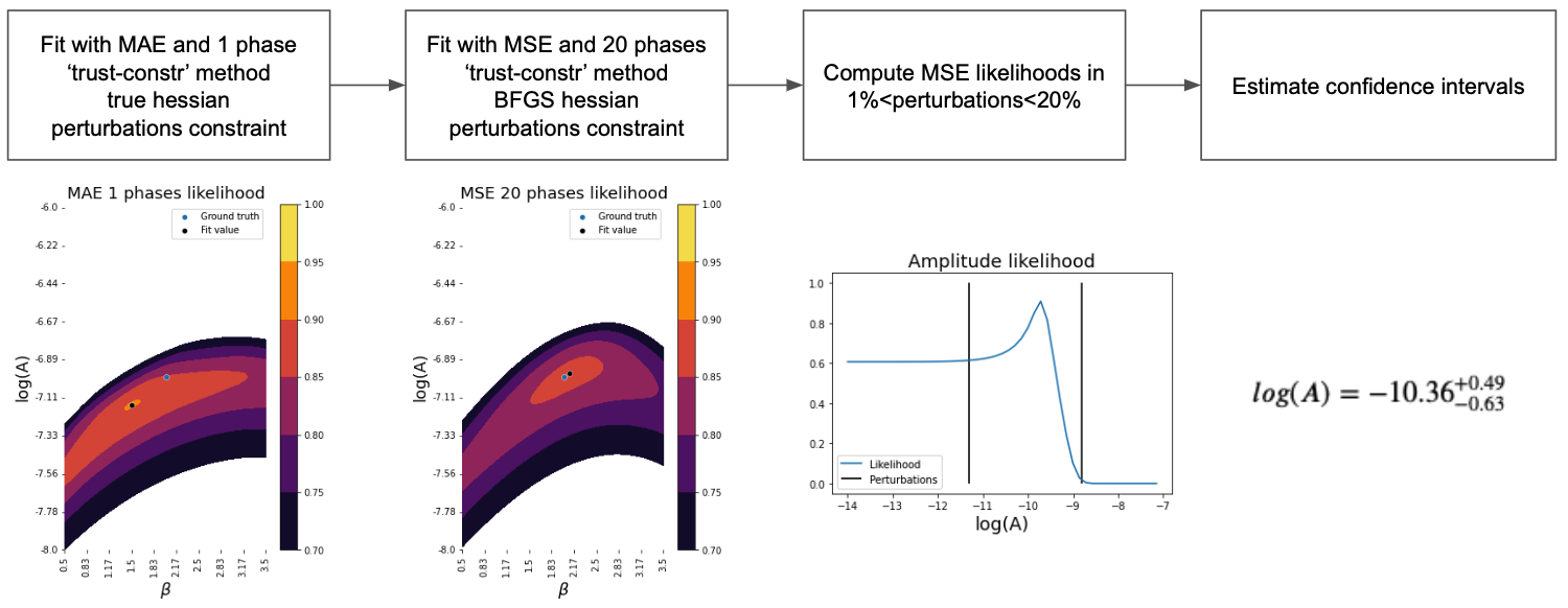
The figure represents the entire pipeline for getting the Amplitude and Power slope of GRF potential perturbations for an observed strong lensing image.
First step: Using MAE loss and only 1 GRF phase approach to the vicinity of the True GRF parameters
Second step: Using MSE loss and 20 GRF phases fine-tune the result getting as close to the True GRF parameters as we can.
Third step: Using the same loss function estimate the likelihood inside the regions of perturbations constraint. This constraint encloses GRFs, whose impact is significant, yet it is still only a perturbation to the main lens.
Fourth step: Out of likelihood in perturbation limits estimate confidence intervals of GRF's Amplitude and Power slope.
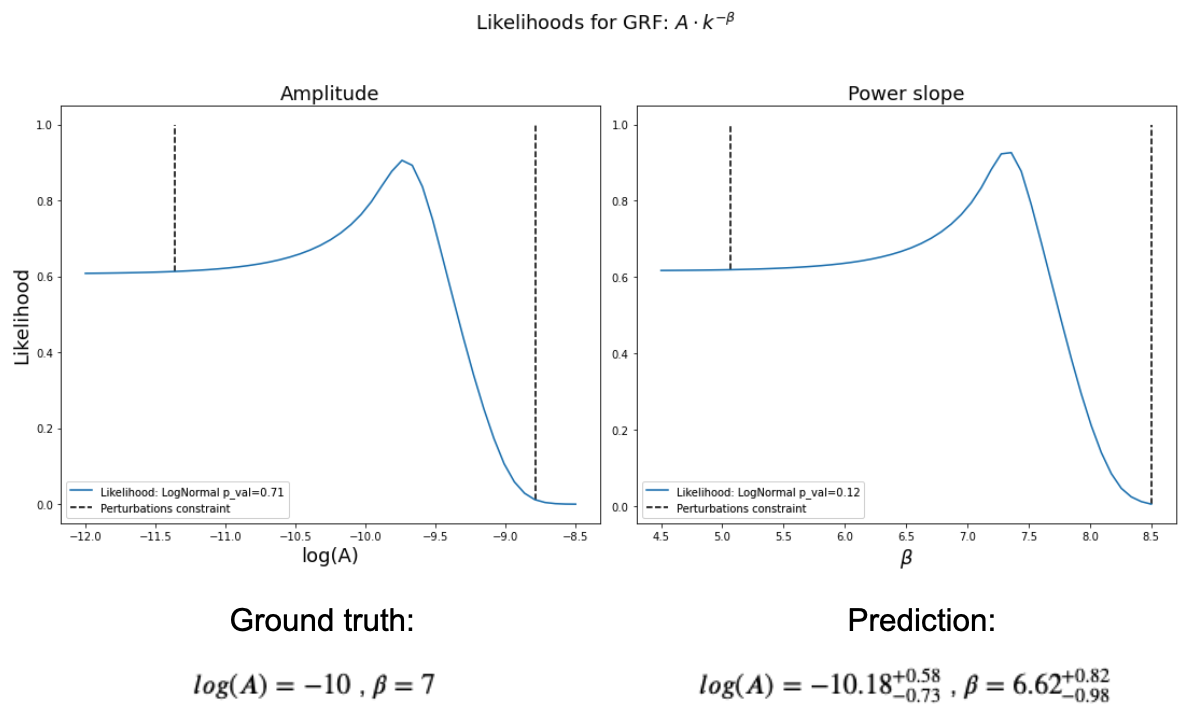
Result likelihoods and GRF parameter estimation for high scale GRF perturbations.
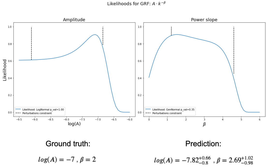
Result likelihoods and GRF parameter estimation for low scale GRF perturbations.
Egor 💻 |
Aymeric 💻 |
Austin 💻 |
