tscluster

This is a project using DVC for setting up a flexible and robust pipeline for clustering subsequences of a time series.

This README explains how to use the pipeline to create predictive models from scratch:

Installation
Setup
Add data
Specify parameters
Run experiments

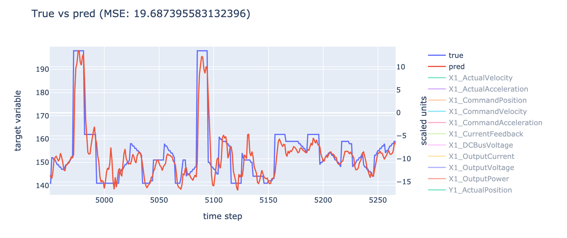
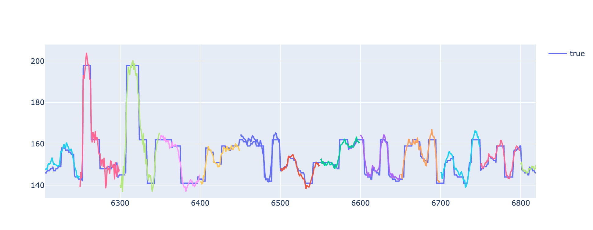
An example of results can be seen here:

Example of results

1. Installation

Developed using Python3.8. You can install the required modules by creating a virtual environment and install the requirements.txt-file (run these commands from the main folder):

mkdir venv
python3 -m venv venv
source venv/bin/activate
pip3 install -r requirements.txt

As an alternative you can install the required modules by running:

pip3 install numpy pandas pandas_profiling matplotlib tensorflow sklearn plotly pyyaml dvc nonconformist shap

To get a plot of the neural network architecture, the following software needs to be installed: Graphviz.

2. Setup DVC

There are 2 options when setting up DVC:

Option A: Simple projects without need for tracking results

Initialize DVC with dvc init --no-scm.

The --no-scm option specifies that we do not want the DVC-related files to be tracked by git, because this repository is agnostic to project-specific things (data files, plots, metrics). This is recommended when there is no need to track experiments in the repository, for simple projects, testing or developing of the pipeline itself.

Option B: Track experiments using git

For long-term projects, it is recommended that you track DVC-related files with git, to take full advantage of the DVC functionality. Follow these steps:

Fork this repository.
Remove the lines under # project-specific files in .gitignore.
Initialize DVC with dvc init.

3. Add data

To add your data to the pipeline, you have two options:

Option A: Place the data files in the folder assets/data/raw/.
Option B: If you want to easily swap between several data sets:
1. Place the files in a subfolder assets/data/raw/[dataset], where dataset is your chosen name of the data
2. In params.yaml, set the parameter dataset to the name of your data set.

Currently only .csv-files are supported.

Example with a data set called data01 (option B):

assets/
├── data/
|   └── raw/
|       ├── data01/
|       |   ├── experiment_01.csv
|       |   ├── experiment_02.csv
|       |   ├── experiment_03.csv
|       |   ├── ...
|       |   ├── experiment_17.csv
|       |   └── experiment_18.csv
|       └─── README.md
├── metrics/
├── plots/
└── profiling/

The data set name is then specified in params.yaml:

profile:
  dataset: data01

...

4. Specify parameters

In params.yaml, specify the name of the target variable (must match the name of the column containing the target variable in the data files). Example with target variable TargetVar:

clean:
    # target: Name of target variable.
    target: TargetVar

The rest of the parameters can also be adjusted. Documentation of the parameters is found in params.yaml.

5. Running experiments

Run experiments by executing this command on the main directory:

dvc repro

On some systems, dvc cannot be run as a standalone command, in which case you will need to run:

python3 -m dvc repro

To run single stages of the pipeline, run:

dvc repro [STAGE NAME]

For example:

dvc repro profile     # will only run the profiling stage
dvc repro featurize   # will only run the featurize stage

Example of results

When the trained model is evaluated, the program produces two plots that visualizes the predictions on the test set. These plots are placed on the folder assets/plots/, and show the following data:

prediction.html: The true target values compared to the predicted target values. Only the first value of each target sequence is used in the plot, and all of this values are connected and plotted as a line. The features used in the model are also plotted.

prediction_sequences.html: Individual predicted target sequences are plotted against the true values. The predicted sequences are shown in different colors to easily distinguish between them. Only a subset of the predicted target sequences are shown, in order to avoid overlapping and make the plot easier to interpret.

ejhusom/tscluster