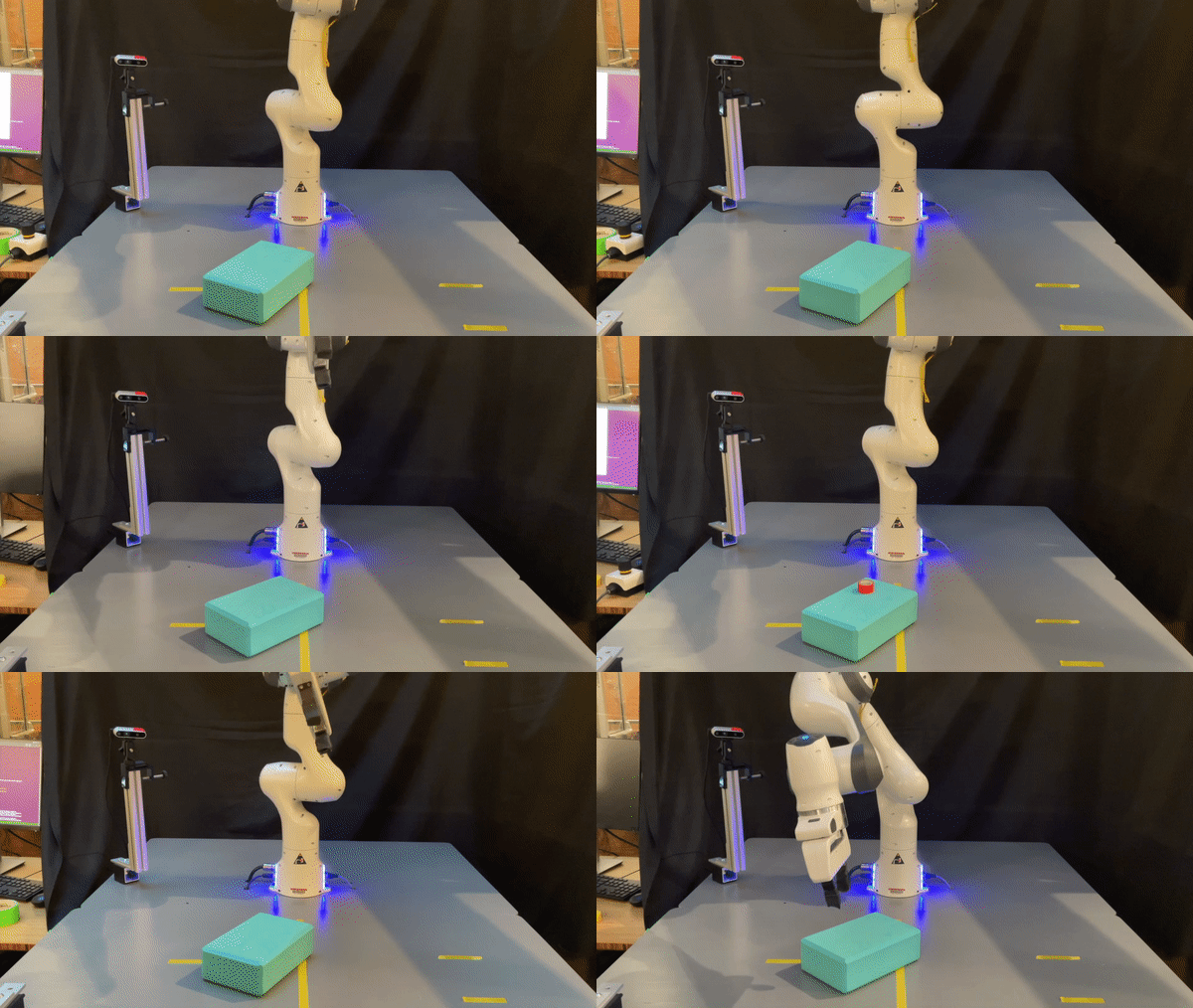
Local Neural Descriptor Fields (LNDF)

PyTorch implementation for training continuous convolutional neural fields to represent dense correspondence across objects, and using these descriptor fields to mimic demonstrations of a pick-and-place task on a robotic system.

This is the reference implementation for our paper:

Local Neural Descriptor Fields: Locally Conditioned Object Representations for Manipulation

PDF | Website

Ethan Chun, Yilun Du, Tomás Lozano-Perez, Leslie Pack Kaelbling

Setup

Clone this repo

git clone --recursive git@github.com:elchun/lndf_robot.git
cd lndf_robot

Create virtual enviroment

If using conda, we recommend python 3.6 although newer python distributions are likely to work as well.

Install dependencies (using a virtual environment is highly recommended):

pip install -e .

If you have installed similar packages before, adding the --no-cache-dir flag may make pip install faster.

pip install -e . --no-cache-dir

Setup additional tools (Franka Panda inverse kinematics -- unnecessary if not using simulated robot for evaluation):

cd pybullet-planning/pybullet_tools/ikfast/franka_panda
python setup.py
cd ../../../../

Setup torch scatter

Install with pip or see additional instructions here. Replace ${CUDA} with the appropriate version (cpu, cu102, cu113, cu116). Generally, the torch and cuda version of torch-scatter should match those of your pytorch installation. E.g. the output of torch.__version__

For example, the authors installed with pip install torch-scatter -f https://data.pyg.org/whl/torch-1.10.1+cu102.html

pip install torch-scatter -f https://data.pyg.org/whl/torch-1.10.1+${CUDA}.html

Setup environment variables

(this script must be sourced in each new terminal where code from this repository is run)

source lndf_env.sh

Quickstart Demo

Download pretrained weights

./scripts/download_weights.sh

Download demos

./scripts/download_demos.sh

Download object data

./scripts/download_obj_data.sh

Run quickstart demo

cd src/ndf_robot/eval

Then open and run quickstart_demo.ipynb. If you are running on a remote server, see here for reference on how to run the jupyter notebook.

Evaluate in Simulation

Download pretrained weights

./scripts/download_demo_weights.sh

Download demos

./scripts/download_demos.sh

Download object data

./scripts/download_obj_data.sh

Run experiment

cd src/ndf_robot/eval
CUDA_VISIBLE_DEVICES=0 python3 evaluate_general.py --config_fname {your_config}

The configuration files are located in the eval_configs directory. Include the .yml extension when specifying the config file.

For example, evaluating a grasping experiment may use the following command:

CUDA_VISIBLE_DEVICES=0 python3 evaluate_general.py --config_fname lndf_grasp.yml

You may create additional experiments by viewing the tutorial.yml config file in src/ndf_robot/eval/eval_configs and creating an appropriate experiment in src/ndf_robot/eval/experiments.

Train Models

Overview

Navigate to the training directory inside ndf_robot. Run or modify the shell script train.sh to train the convolutional occupancy network.

Two main scripts control how the model is trained: train_conv_occupancy_net.py and losses.py. The shell script calls train_conv_occupancy_net.py which allows the user to specify the model and loss function to use. These loss functions are defined in losses.py. A user may use the given loss functions or test additional loss functions

To evaluate a new set of weights, the s_vis_correspondance.py script is convenient. By setting the model_path and obj_model variables, you can compare the latent representation of an unrotated and rotated version of the same object. This allows you to check how strongly SE(3) equivariance is enforced.

Loss functions

Four main loss functions are defined in losses.py. The first two occupancy_net losses are used for training a standard occupancy network or a convolutional occupancy network. The latter two contrastive loss functions implement the distance based loss function which we describe in our publication. We find that the contrastive_cross_entropy loss performs the best, while the contrastive_l2 loss works but produces lower success rates.

Both contrastive loss functions select a sample point, $x_0$ and a set of target points ${x_i}$. To enforce SE(3) equivariance, we compare the latent codes of these points on a rotated and unrotated object. More specifically, we calculate the cosine similarity between the latent code of the sample point on an unrotated object and the latent code of the target points on the rotated object. We would like target points closer to the sample point to have more similar latent codes.

Contrastive Cross Entropy

In contrastive_cross_entropy loss, we enforce this similarity by calculating the euclidean distance between the sample and target points (assuming both are on the same mug). We then produce a probability distribution where the probability assigned to a target point is

$$ p_i = \frac{1 / (d_i + \epsilon)}{\sum_j{1/(d_j + \epsilon)}} $$

where $d_i$ is the distance between the sample and target points and $\epsilon$ is a constant set prior to training which dictates how sharply $p_i$ increases as the target points get closer to the sample point. We then consider this loss as a prediction problem where the cosine similarity between $x_0$ and $x_i$ predicts that $x_i = x_0$ with probability $p_i$.

Contrastive L2

In contrastive_l2 loss, we also calculate the euclidean distance between the sample and target points. However, for each target point $x_i$, we instead create a target value $t_i$ defined by

$$ t_i = 2*\exp({-d_i^2 * \frac{\ln{2}}{r^2}}) - 1 $$

Where $d_i$ is the distance between $x_i$ and $x_0$ and $r$ is a constant that defines the steepness of this distribution. This function enforces an exponential decay as a function of $d_i$ where $r$ is the distance at which $t_i = 0$. Additionally, this function is bound between 1 and -1.

We calculate then drive the cosine similarity of the latent code of $x_0$ and $x_i$ to this $t_i$ value using L2 loss.

Add demonstrations

Navigate to the demonstrations directory inside ndf_robot. Use the label_demos.py script to log new demonstrations. The current evaluator uses a slightly different file format than the output of label_demos.py so you must run the convert_demos.py script to convert the demonstrations into the new file format.

Advanced Changes

Add or modify models: Use the descriptions directory to modify or add new models.
Modify optimizer: See both the deep or geometric optimizer classes in the opt directory.

Data Generation

Download all the object data assets

./scripts/download_obj_data.sh

Run data generation

cd src/ndf_robot/data_gen
python shapenet_pcd_gen.py \
    --total_samples 100 \
    --object_class mug \
    --save_dir test_mug \
    --rand_scale \
    --num_workers 2

More information on dataset generation can be found here.

Collect new demonstrations with teleoperated robot in PyBullet

Make sure you have downloaded all the object data assets (see Data Generation section)

Run teleoperation pipeline

cd src/ndf_robot/demonstrations
python label_demos.py --exp test_bottle --object_class bottle --with_shelf

More information on collecting robot demonstrations can be found here.

Citing

If you find our paper or this code useful in your work, please cite our paper:

@article{chundu2023lndf,
  title = {Local Neural Descriptor Fields: Locally Conditioned Object Representations for Manipulation},
  author = {Chun, Ethan and Du, Yilun and Simeonov, Anthony and Lozano-Perez, Tomas and Kaelbling, Leslie},
  journal = {arXiv preprint arXiv:2302.03573},
  year = {2023}
}

Acknowledgements

Parts of this code were built upon the implementations found in the convolutional occupancy networks repo, the neural descriptor field repo, the occupancy networks repo and the vector neurons repo. Check out their projects as well!