Simple/limited/incomplete benchmark for scalability, speed and accuracy of machine learning libraries for classification
This project aims at a minimal benchmark for scalability, speed and accuracy of commonly used implementations of a few machine learning algorithms. The target of this study is binary classification with numeric and categorical inputs (of limited cardinality i.e. not very sparse) and no missing data, perhaps the most common problem in business applications (e.g. credit scoring, fraud detection or churn prediction). If the input matrix is of n x p, n is varied as 10K, 100K, 1M, 10M, while p is ~1K (after expanding the categoricals into dummy variables/one-hot encoding). This particular type of data structure/size (the largest) stems from this author's interest in some particular business applications.
The algorithms studied are
- linear (logistic regression, linear SVM)
- random forest
- boosting
- deep neural network
in various commonly used open source implementations like
- R packages
- Python scikit-learn
- Vowpal Wabbit
- H2O
- xgboost
- Spark MLlib.
(Update: It turns out these are the most popular tools used for machine learning indeed. If your software tool of choice is not here, your can benchmark it with minimal work with the following instructions.)
Random forest, boosting and more recently deep neural networks are the algos expected to perform the best on the structure/sizes described above (e.g. vs alternatives such as k-nearest neighbors, naive-Bayes, decision trees, linear models etc). Non-linear SVMs are also among the best in accuracy in general, but become slow/cannot scale for the larger n sizes we want to deal with. The linear models are less accurate in general and are used here only as a baseline (but they can scale better and some of them can deal with very sparse features).
By scalability we mean here that the algos are able to complete (in decent time) for the given data sizes with the main constraint being RAM (a given algo/implementation will crash if running out of memory). Some of the algos/implementations can work in a distributed setting, although the largest dataset in this study n = 10M is less than 1GB, so scaling out to multiple machines should not be necessary and is not the focus of this current study. (Also, some of the algos perform relatively poorly speedwise in the multi-node setting, where communication is over the network rather than via updating shared memory.) Speed (in the single node setting) is determined by computational complexity but also if the algo/implementation can use multiple processor cores. Accuracy is measured by AUC. The interpretability of models is not of concern in this project.
In summary, we are focusing on which algos/implementations can be used to train relatively accurate binary classifiers for data with millions of observations and thousands of features processed on commodity hardware (mainly one machine with decent RAM and several cores).
Training datasets of sizes 10K, 100K, 1M, 10M are generated from the well-known airline dataset (using years 2005 and 2006). A test set of size 100K is generated from the same (using year 2007). The task is to predict whether a flight will be delayed by more than 15 minutes. While we study primarily the scalability of algos/implementations, it is also interesting to see how much more information and consequently accuracy the same model can obtain with more data (more observations).
The tests have been carried out on a Amazon EC2 c3.8xlarge instance (32 cores, 60GB RAM). The tools are freely available and their installation is trivial (version information here). For some of the models that ran out of memory for the larger data sizes a r3.8xlarge instance (32 cores, 250GB RAM) has been used occasionally. For deep learning on GPUs, a g2.8xlarge (4 GPUs with 4GB video memory each, 32 CPU cores, 60GB RAM) instance has been used.
Note: This project is still work in progress, the results presented here on github are "as they are coming in". A more digested version of the results (at least including LR, RF, GBM and "big data") can be found in a talk at the Los Angeles Machine Learning meetup: slides and video.
For each algo/tool and each size n we observe the following: training time, maximum memory usage during training, CPU usage on the cores, and AUC as a measure for predictive accuracy. Times to read the data, pre-process the data, score the test data are also observed but not reported (not the bottleneck).
The linear models are not the primary focus of this study because of their not so great accuracy vs the more complex models (on this type of data). They are analysed here only to get some sort of baseline.
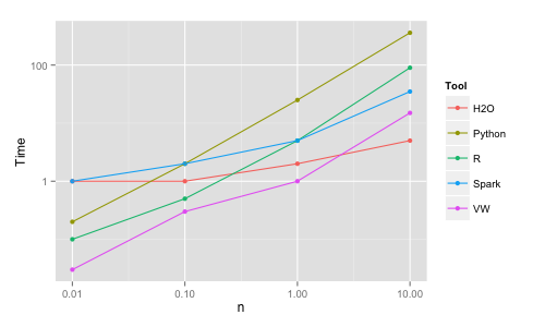
The R glm package (the basic R tool for logistic regression) is very slow, 500 seconds on n = 0.1M (AUC 70.6). Therefore, for R the glmnet package is used. For Python/scikit-learn LogisticRegression (based on the LIBLINEAR C++ library) has been used.
| Tool | n | Time (sec) | RAM (GB) | AUC |
|---|---|---|---|---|
| R | 10K | 0.1 | 1 | 66.7 |
    | 100K |      0.5      |   1      | 70.3
    | 1M   |      5        |   1      | 71.1
    | 10M  |      90       |   5      | 71.1
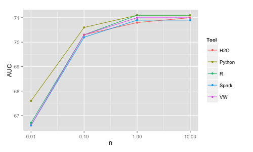
Python | 10K | 0.2 | 2 | 67.6 | 100K | 2 | 3 | 70.6 | 1M | 25 | 12 | 71.1 | 10M | crash/360 | | 71.1 VW | 10K | 0.3 (/10) | | 66.6 | 100K | 3 (/10) | | 70.3 | 1M | 10 (/10) | | 71.0 | 10M | 15 | | 71.0 H2O | 10K | 1 | 1 | 69.6 | 100K | 1 | 1 | 70.3 | 1M | 2 | 2 | 70.8 | 10M | 5 | 3 | 71.0 Spark | 10K | 1 | 1 | 66.6 | 100K | 2 | 1 | 70.2 | 1M | 5 | 2 | 70.9 | 10M | 35 | 10 | 70.9
Python crashes on the 60GB machine, but completes when RAM is increased to 250GB (using a sparse format would help with memory footprint and likely runtime as well). The Vowpal Wabbit (VW) running times are reported in the table for 10 passes (online learning) over the data for the smaller sizes. While VW can be run on multiple cores (as multiple processes communicating with each other), it has been run here in the simplest possible way (1 core). Also keep in mind that VW reads the data on the fly while for the other tools the times reported exclude reading the data into memory.
One can play with various parameters (such as regularization) and even do some search in the parameter space with cross-validation to get better accuracy. However, very quick experimentation shows that at least for the larger sizes regularization does not increase accuracy significantly (which is expected since n >> p).
The main conclusion here is that it is trivial to train linear models even for n = 10M rows virtually in any of these tools on a single machine in a matter of seconds. H2O and VW are the most memory efficient (VW needs only 1 observation in memory at a time therefore is the ultimately scalable solution). H2O and VW are also the fastest (for VW the time reported includes the time to read the data as it is read on the fly). Again, the differences in memory efficiency and speed will start to really matter only for larger sizes and beyond the scope of this study.
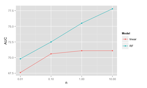
For this dataset the accuracy of the linear model tops-off at moderate sizes while the accuracy of non-linear models (e.g. random forest) continues to increase with increasing data size. This is because a simple linear structure can be extracted already from a smaller dataset and having more data points will not change the classification boundary significantly. On the other hand, more complex models such as random forests can improve further with increasing data size by adjusting further the classification boundary.
This means that having more data ("big data") does not improve further the accuracy of the linear model (at least for this dataset).
Note also that the random forest model is more accurate than the linear one for any size, and contrary to the conventional wisdom of "more data beats better algorithms", the random forest model on 1% of the data (100K records) beats the linear model on all the data (10M records).
Similar behavior can be observed in other non-sparse datasets, e.g. the Higgs dataset. Contact me (e.g. submit a github issue) if you have learning curves for linear vs non-linear models on other datasets (dense or sparse).
On the other hand, there is certainly a price for higher accuracy in terms of larger required training (CPU) time.
Ultimately, there is a data size - algo (complexity) - cost (CPU time) - accuracy tradeoff (to be studied in more details later). Some quick results for H2O:
| n | Model | Time (sec) | AUC |
|---|---|---|---|
| 10M | Linear | 5 | 71.0 |
| 0.1M | RF | 150 | 72.5 |
| 10M | RF | 4000 | 77.8 |
Note: The random forests results have been published in a more organized and self-contained form in this blog post.
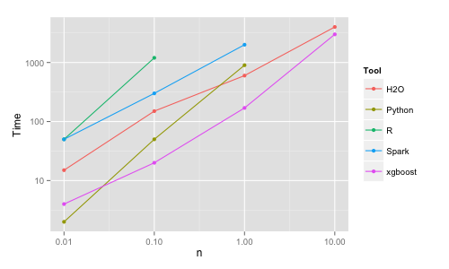
Random forests with 500 trees have been trained in each tool choosing the default of square root of p as the number of variables to split on.
| Tool | n | Time (sec) | RAM (GB) | AUC |
|---|---|---|---|---|
| R | 10K | 50 | 10 | 68.2 |
    | 100K |     1200      |   35     | 71.2
    | 1M   |     crash     |          |
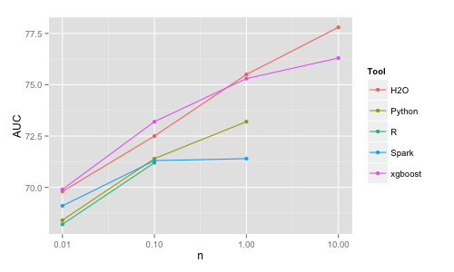
Python | 10K | 2 | 2 | 68.4 | 100K | 50 | 5 | 71.4 | 1M | 900 | 20 | 73.2 | 10M | crash | | H2O | 10K | 15 | 2 | 69.8 | 100K | 150 | 4 | 72.5 | 1M | 600 | 5 | 75.5 | 10M | 4000 | 25 | 77.8 Spark | 10K | 50 | 10 | 69.1 | 100K | 270 | 30 | 71.3 | 1M | crash/2000 | | 71.4 xgboost | 10K | 4 | 1 | 69.9 | 100K | 20 | 1 | 73.2 | 1M | 170 | 2 | 75.3 | 10M | 3000 | 9 | 76.3
The R implementation (randomForest package) is slow and inefficient in memory use. It cannot cope by default with a large number of categories, therefore the data had to be one-hot encoded. The implementation uses 1 processor core, but with 2 lines of extra code it is easy to build the trees in parallel using all the cores and combine them at the end. However, it runs out of memory already for n = 1M. I have to emphasize this has nothing to do with R per se (and I still stand by arguing R is the best data science platform esp. when it comes to data munging of structured data or visualization), it is just this particular (C and Fortran) RF implementation used by the randomForest package that is inefficient.
The Python (scikit-learn) implementation is faster, more memory efficient and uses all the cores. Variables needed to be one-hot encoded (which is more involved than for R) and for n = 10M doing this exhausted all the memory. Even if using a larger machine with 250GB of memory (and 140GB free for RF after transforming all the data) the Python implementation runs out of memory and crashes for this larger size. The algo finished successfully though when run on the larger box with simple integer encoding (which for some datasets/cases might be actually a good approximation/choice).
The H2O implementation is fast, memory efficient and uses all cores. It deals with categorical variables automatically. It is also more accurate than the studied R/Python packages, which may be because of dealing properly with the categorical variables, i.e. internally in the algo rather than working from a previously 1-hot encoded dataset (where the link between the dummies belonging to the same original variable is lost).
Spark (MLlib) implementation is slower and has a larger memory footprint.
It runs out of memory already at n = 1M (with 250G of RAM it finishes for n = 1M,
but it crashes for n = 10M). However, as Spark
can run on a cluster one can throw in even more RAM by using more nodes.
I also tried to provide the categorical
variables encoded simply as integers and passing the categoricalFeaturesInfo parameter, but that made
training much slower.
A convenience issue, reading the data is more than one line of code and at the start of this benchmark project
Spark did not provide a one-hot encoder
for the categorical data (therefore I used R for that). This has been ammended since, thanks @jkbradley
for native 1-hot encoding code.
In earlier versions of this benchmark there was an issue of Spark random forests having
low prediction accuracy vs the other methods. This was due to aggregating votes rather than probabilities
and it has been addressed by @jkbradley in this
code (will be included in next Spark release).
There is still an open issue on the accuracy for n = 1M (see the breaking trend in the AUC graph).
To get more insights on the issues above see
more comments
by Joseph Bradley @jkbradley of Databricks/Spark project (thanks, Joseph).
I also tried xgboost, a popular library for boosting which is capable to build random forests as well. It is fast, memory efficient and of high accuracy. Note the different shapes of the AUC and runtime vs dataset size curves for H2O and xgboost, some discussions here.
Both H2O and xgboost have interfaces from R and Python.
A few other RF implementations (open source and commercial as well) have been benchmarked quickly on 1M records and runtime and AUC are reported here.
It would be nice to study the dependence of running time and accuracy as a function of the (hyper)parameter values of the algorithm, but a quick idea can be obtained easily for the H2O implementation from this table (n = 10M on 250GB RAM):
| ntree | depth | nbins | mtries | Time (hrs) | AUC |
|---|---|---|---|---|---|
| 500 | 20 | 20 | -1 (2) | 1.2 | 77.8 |
| 500 | 50 | 200 | -1 (2) | 4.5 | 78.9 |
| 500 | 50 | 200 | 3 | 5.5 | 78.9 |
| 5000 | 50 | 200 | -1 (2) | 45 | 79.0 |
| 500 | 100 | 1000 | -1 (2) | 8.3 | 80.1 |
other hyperparameters being sample rate (at each tree), min number of observations in nodes, impurity function.
One can see that the AUC could be improved further and the best AUC from this dataset with random forests seems to be around 80 (the best AUC from linear models seems to be around 71, and we will compare with boosting and deep learning later).
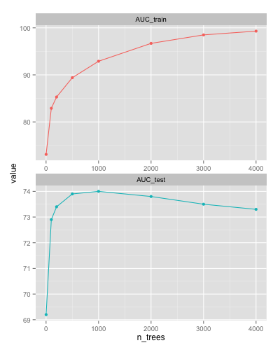
Compared to random forests, GBMs have a more complex relationship between hyperparameters and accuracy (and also runtime). The main hyperparameters are learning (shrinkage) rate, number of trees, max depth of trees, while some others are number of bins, sample rate (at each tree), min number of observations in nodes. To add to complexity, GBMs can overfit in the sense that adding more trees at some point will result in decreasing accuracy on a test set (while on the training set "accuracy" keeps increasing).
For example using xgboost for n = 100K learn_rate = 0.01 max_depth = 16 (and the
printEveryN = 100 and eval_metric = "auc" options) the AUC on the train and test sets,
respectively after n_trees number of iterations are:
One can see the AUC on the test set decreases after 1000 iterations (overfitting).
xgboost has a handy early stopping option (early_stop_round = k - training
will stop if performance e.g. on a holdout set keeps getting worse consecutively
for k rounds). If one does not know where to stop, one might underfit (too few iterations)
or overfit (too many iterations) and the resulting model will be suboptimal in accuracy
(see Fig. above).
Doing an extensive search for the best model is not the main goal of this project. Nevertheless, a quick exploratory search in the hyperparameter space has been conducted using xgboost (with the early stopping option). For this a separate validation set of size 100K from 2007 data not used in the test set has been generated. The goal is to find parameter values that provide decent accuracy and then run all GBM implementations (R, Python scikit-learn, etc) with those parameter values to compare speed/scalability (and accuracy).
The smaller the learn_rate the better the AUC, but for very small values training time increases dramatically,
therefore we use learn_rate = 0.01 as a compromise.
Unlike recommended in much of the literature, shallow trees don't produce best (or close to best) results,
the grid search showed better accuracy e.g. with max_depth = 16.
The number of trees to produce optimal results for the above hyperparameter values depend though on the training set size.
For n_trees = 1000 we don't reach the overfitting regime
for either size and we use this value for studying the speed/scalability of the different implementations.
(Values for the other hyper-parameters that seem to work well are:
sample_rate = 0.5 min_obs_node = 1.) We call this experiment A (in the table below).
Unfortunately some implementations take too much time to run for the above parameter values
(and Spark runs out of memory). Therefore, another set of parameter values (that provide lower accuracy but faster training times)
has been also used to study speed/scalability: learn_rate = 0.1 max_depth = 6 n_trees = 300.
We call this experiment B.
I have to emphasize that while I make the effort to match parameter values for all algos/implementations, every implementation is different, some don't have all the above parameters, while some might use the existing ones in a slightly different way (you can also see the resulting model/AUC is somewhat different). Nevertheless, the results below give us a pretty good idea of how the implementations compare to each other.
| Tool | n | Time (s) A | Time (s) B | AUC A | AUC B | RAM(GB) A | RAM(GB) B |
|---|---|---|---|---|---|---|---|
| R | 10K | 20 | 3 | 64.9 | 63.1 | 1 | 1 |
    | 100K |   200         |   30       |   72.3 |  71.6  |    1      |     1
    | 1M   |   3000        |   400      |   74.1 |  73.9  |    1      |     1
    | 10M  |               |   5000     |        |  74.3  |           |     4
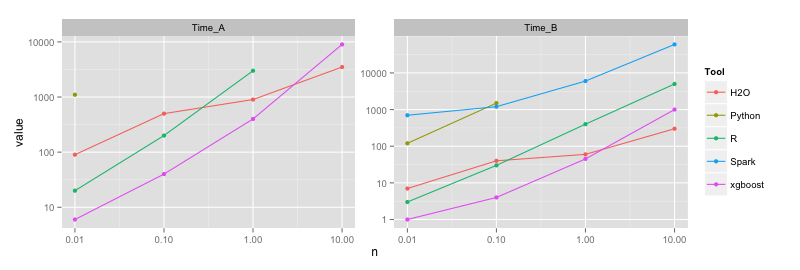
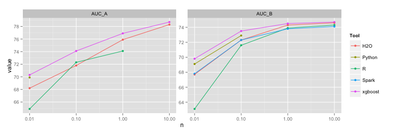
Python | 10K | 1100 | 120 | 69.9 | 69.1 | 2 | 2 | 100K | | 1500 | | 72.9 | | 3 | 1M | | | | | | | 10M | | | | | | H2O | 10K | 90 | 7 | 68.2 | 67.7 | 3 | 2 | 100K | 500 | 40 | 71.8 | 72.3 | 3 | 2 | 1M | 900 | 60 | 75.9 | 74.3 | 9 | 2 | 10M | 3500 | 300 | 78.3 | 74.6 | 11 | 20 Spark | 10K | 180000 | 700 | 66.4 | 67.8 | 30 | 10 | 100K | | 1200 | | 72.3 | | 30 | 1M | | 6000 | | 73.8 | | 30 | 10M | | (60000) | | (74.1) | | crash (110) xgboost | 10K | 6 | 1 | 70.3 | 69.8 | 1 | 1 | 100K | 40 | 4 | 74.1 | 73.5 | 1 | 1 | 1M | 400 | 45 | 76.9 | 74.5 | 1 | 1 | 10M | 9000 | 1000 | 78.7 | 74.7 | 6 | 5
The memory footprint of GBMs is in general smaller than for random forests, therefore the bottleneck is mainly training time (although besides being slow Spark is inefficient in memory use as well especially for deeper trees, therefore it crashes).
Similar to random forests, H2O and xgboost are the fastest (both use multithreading). R does relatively well considering that it's a single-threaded implementation. Python is very slow with one-hot encoding of categoricals, but almost as fast as R (just 1.5x slower) with simple/integer encoding. Spark is slow and memory inefficient, but at least for shallow trees it achieves similar accuracy to the other methods (unlike in the case of random forests or logistic regression, where Spark provides lower accuracy than its peers).
Compared to random forests, boosting requires more tuning to get a good choice of hyperparameters.
Quick results for H2O and xgboost with n = 10M (largest data)
learn_rate = 0.01 (the smaller the better
AUC, but also longer and longer training times) max_depth = 20 (after rough search with
max_depth = 2,5,10,20,50) n_trees = 5000 (close to xgboost early stop)
min_obs_node = 1 (and sample_rate = 0.5 for xgboost, n_bins = 1000 for H2O):
| Tool | Time (hr) | AUC |
|---|---|---|
| H2O | 7.5 | 79.8 |
| H2O-3 | 9.5 | 81.2 |
| xgboost | 14 | 81.1 |
Compare with H2O random forest from previous section (Time 8.3 hr, AUC 80.1). H2O-3 is the new generation/version of H2O.
...
While my primary interest is in machine learning on datasets of 10M records, you might be interested in larger datasets. Some problems might need a cluster, though there has been a tendency recently to solve every problem with distributed computing, needed or not. As a reminder, sending data over a network vs using shared memory is a big speed difference. Also several popular distributed systems have significant computation and memory overhead, and more fundamentally, their communication patterns (e.g. map-reduce style) are not the best fit for many of the machine learning algos.
For linear models, most tools, including single-core R work well on 100M records still on a single server (r3.8xlarge instance with 32 cores, 250GB RAM used here). (A 10x copy of the 10M dataset has been used, therefore information on AUC vs size is invalid and is not considered here.)
Linear models, 100M rows:
| Tool | Time[s] | RAM[GB] |
|---|---|---|
| R | 1000 | 60 |
| Spark | 160 | 120 |
| H2O | 40 | 20 |
| VW | 150 |
Some tools can handle 1B records on a single machine (in fact VW never runs out of memory, so if larger runtimes are acceptable, you can go further still on one machine).
Linear models, 1B rows:
| Tool | Time[s] | RAM[GB] |
|---|---|---|
| H2O | 500 | 100 |
| VW | 1400 |
For tree-based ensembles (RF, GBM) H2O and xgboost can train on 100M records on a single server, though the training times become several hours:
RF/GBM, 100M rows:
| Algo | Tool | Time[s] | Time[hr] | RAM[GB] |
|---|---|---|---|---|
| RF | H2O | 40000 | 11 | 80 |
| xgboost | 36000 | 10 | 60
GBM | H2O | 35000 | 10 | 100
| xgboost | 110000 | 30 | 50
One usually hopes here (and most often gets) much better accuracy for the 1000x in training time vs linear models.
Some quick results:
H2O logistic runtime (sec):
| 1 node | 5 nodes
--------|---------|---------- 100M | 42 | 9.9 1B | 480 | 101
H2O RF runtime (sec) (5 trees):
| 1 node | 5 nodes
--------|---------|----------
10M | 42 | 41
100M | 405 | 122
...
