absmapsdata

The absmapsdata package exists to make it easier to produce maps from ABS data in R. The package contains compressed, tidied, and lazily-loadable sf objects containing geometric information about ABS data structures.

Before we get into the ‘what problem is this package solving’ details, let’s look at some examples so that you can copy-paste into your own script and replicate out-of-the-box (and impress your friends).

Installation

You can install absmapsdata from github with:

# install.packages("devtools")
devtools::install_github("wfmackey/absmapsdata")

The sf package is required to handle the sf objects:

# install.packages("sf")
library(sf)

And we will use the tidyverse packages in this example:

# install.packages("tidyverse")
library(tidyverse)

Maps loaded with this package

Available maps are listed below. These will be added to over time. If you would like to request a map to be added, let me know via an issue on this Github repo. (Or send me an email: wfmackey@gmail.com)

ASGS Main Structures

Statistical Area 1 2011: sa12011
Statistical Area 1 2016: sa12016
Statistical Area 2 2011: sa22011
Statistical Area 2 2016: sa22016
Statistical Area 3 2011: sa32011
Statistical Area 3 2016: sa32016
Statistical Area 4 2011: sa42011
Statistical Area 4 2016: sa42016
Greater Capital Cities 2011: gcc2011
Greater Capital Cities 2016: gcc2016
Remoteness Areas 2011: ra2011
Remoteness Areas 2016: ra2016
State 2011: state2011
State 2016: state2016

ASGS Non-ABS Structures

Commonwealth Electoral Divisions 2018: ced2018
State Electoral Divisions 2018:sed2018
Local Government Areas 2016: lga2016
Local Government Areas 2018: lga2018

Just show me how to make a map with this package

Using the package’s pre-loaded data

The absmapsdata package comes with pre-downloaded and pre-processed data. To load a particular geospatial object, simply load the package and call the object:

library(absmapsdata)

mapdata1 <- sa32011

glimpse(mapdata1)
#> Observations: 351
#> Variables: 12
#> $ sa3_code_2011   <chr> "10101", "10102", "10103", "10104", "10201", "10…
#> $ sa3_name_2011   <chr> "Goulburn - Yass", "Queanbeyan", "Snowy Mountain…
#> $ sa4_code_2011   <chr> "101", "101", "101", "101", "102", "102", "103",…
#> $ sa4_name_2011   <chr> "Capital Region", "Capital Region", "Capital Reg…
#> $ gcc_code_2011   <chr> "1RNSW", "1RNSW", "1RNSW", "1RNSW", "1GSYD", "1G…
#> $ gcc_name_2011   <chr> "Rest of NSW", "Rest of NSW", "Rest of NSW", "Re…
#> $ state_code_2011 <chr> "1", "1", "1", "1", "1", "1", "1", "1", "1", "1"…
#> $ state_name_2011 <chr> "New South Wales", "New South Wales", "New South…
#> $ albers_sqkm     <dbl> 21236.6140, 6511.1214, 14281.8301, 9864.9397, 98…
#> $ cent_lat        <dbl> 149.0763, 149.6013, 148.9416, 149.8063, 151.2182…
#> $ cent_long       <dbl> -34.55399, -35.44940, -36.43958, -36.49934, -33.…
#> $ geometry        <MULTIPOLYGON [°]> MULTIPOLYGON (((149.1198 -3..., MUL…

mapdata2 <- sa22016

glimpse(mapdata2)
#> Observations: 2,310
#> Variables: 15
#> $ sa2_main_2016   <chr> "101021007", "101021008", "101021009", "10102101…
#> $ sa2_5dig_2016   <chr> "11007", "11008", "11009", "11010", "11011", "11…
#> $ sa2_name_2016   <chr> "Braidwood", "Karabar", "Queanbeyan", "Queanbeya…
#> $ sa3_code_2016   <chr> "10102", "10102", "10102", "10102", "10102", "10…
#> $ sa3_name_2016   <chr> "Queanbeyan", "Queanbeyan", "Queanbeyan", "Quean…
#> $ sa4_code_2016   <chr> "101", "101", "101", "101", "101", "101", "101",…
#> $ sa4_name_2016   <chr> "Capital Region", "Capital Region", "Capital Reg…
#> $ gcc_code_2016   <chr> "1RNSW", "1RNSW", "1RNSW", "1RNSW", "1RNSW", "1R…
#> $ gcc_name_2016   <chr> "Rest of NSW", "Rest of NSW", "Rest of NSW", "Re…
#> $ state_code_2016 <chr> "1", "1", "1", "1", "1", "1", "1", "1", "1", "1"…
#> $ state_name_2016 <chr> "New South Wales", "New South Wales", "New South…
#> $ areasqkm_2016   <dbl> 3418.3525, 6.9825, 4.7634, 13.0034, 3054.4099, 1…
#> $ cent_lat        <dbl> 149.7932, 149.2328, 149.2255, 149.2524, 149.3911…
#> $ cent_long       <dbl> -35.45508, -35.37590, -35.35103, -35.35520, -35.…
#> $ geometry        <MULTIPOLYGON [°]> MULTIPOLYGON (((149.7606 -3..., MUL…

The resulting sf object contains one observation per area (in the following examples, one observation per sa3). It stores the geometry information in the geometry variable, which is a nested list describing the area’s polygon. The object can be joined to a standard data.frame or tibble and can be used with dplyr functions.

Creating maps with your `sf` object

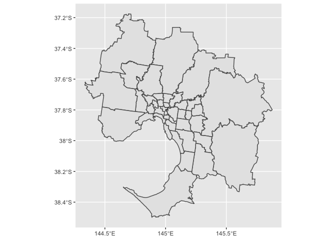
We do all this so we can create gorgeous maps. And with the sf object in hand, plotting a map via ggplot and geom_sf is simple.

map <-
sa32016 %>%
  filter(gcc_name_2016 == "Greater Melbourne") %>%   # let's just look Melbourne
  ggplot() +
  geom_sf(aes(geometry = geometry))  # use the geometry variable

map

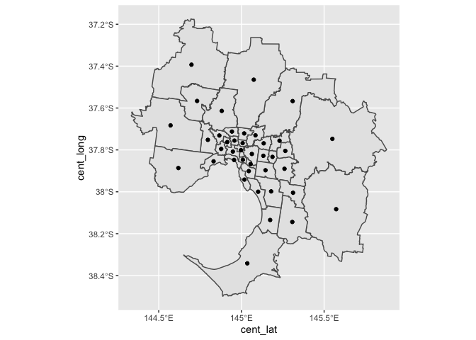
The data also include centorids of each area, and we can add these points to the map with the cent_lat and cent_long variables using geom_point.

map <-
sa32016 %>%
  filter(gcc_name_2016 == "Greater Melbourne") %>%   # let's just look Melbourne
  ggplot() +
  geom_sf(aes(geometry = geometry)) +   # use the geometry variable
  geom_point(aes(cent_lat, cent_long))  # use the centroid lat and longs

map

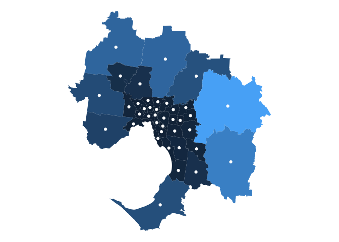
Cool. But, sidenote, this all looks a bit ugly. We can pretty it up using ggplot tweaks. See the comments on each line for its objective. Also note that we’re filling the areas by their areasqkm size, another variable included in the sf object (we’ll replace this with more interesting data in the next section).

map <-
sa32016 %>%
  filter(gcc_name_2016 == "Greater Melbourne") %>%   # let's just look Melbourne
  ggplot() +
  geom_sf(aes(geometry = geometry,  # use the geometry variable
              fill = areasqkm_2016),     # fill by area size
          lwd = 0,                  # remove borders
          show.legend = FALSE) +    # remove legend
  geom_point(aes(cent_lat,
                 cent_long),        # use the centroid lat and longs
             colour = "white") +    # make the points white
  theme_void() +                    # clears other plot elements
  coord_sf(datum = NA)              # fixes a gridline bug in theme_void()

map

Joining with other datasets

At some point, we’ll want to join our spatial data with data-of-interest. The variables in our mapping data—stating the numeric code and name of each area and parent area—will make this relatively easy.

For example: suppose we had a simple dataset of median income by SA3 over time.

# Read data in some data
income <- read_csv("data/median_income_sa3.csv")

#> Parsed with column specification:
#> cols(
#>   sa3_name_2016 = col_character(),
#>   year = col_character(),
#>   median_income = col_double()
#> )

This income data contains a variable sa3_name_2016, and we can use dplyr::left_join() to combine with our mapping data.

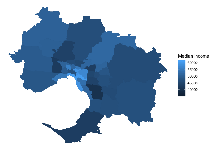
combined_data <- left_join(income, sa32016, by = "sa3_name_2016")

Now that we have a tidy dataset with 1) the income data we want to plot, and 2) the geometry of the areas, we can plot income by area:

map <-
combined_data %>%
  filter(gcc_name_2016 == "Greater Melbourne") %>%   # let's just look Melbourne
  ggplot() +
  geom_sf(aes(geometry = geometry,  # use the geometry variable
              fill = median_income),        # fill by unemployment rate
          lwd = 0) +                # remove borders
  theme_void() +                    # clears other plot elements
  coord_sf(datum = NA) +            # fixes a gridline bug in theme_void()
  labs(fill = "Median income")

map

Why does this package exist?

The motivation for this package is that maps are cool and fun and are, sometimes, the best way to communicate data. And making maps is R with ggplot is relatively easy when you have the right object.

Getting the right object is not technically difficult, but requires research into the best-thing-to-do at each of the following steps:

Find the ASGS ABS spatial-data page and determine the right file to download.
Read the shapefile into R using one-of-many import tools.
Convert the object into something usable.
Clean up any inconsistencies and apply consistent variable naming/values across areas and years.
Find an appropriate compression function and level to optimise output.

For me, at least, finding the correct information and developing the best set of steps was a little bit interesting but mostly tedious and annoying. The absmapsdata package holds this data for you, so you can spend more time making maps, and less time on Stack Overflow, the ABS website, and lovely-people’s wonderful blogs.

How does this package do the-things-it-does

The absmapsdata package simple holds compressed and easy to use data (sf objects) for you use.

It is a data-only-based sibling of absmaps, which holds functionality to download more shapefile data from the ABS and compress it to a level you desire. However, this comes at a cost: the mapping software that absmaps is built on can be a bit fiddly to install.

If you would like to do these things, please feel free to install absmapsdata.

I want to complain about this package

Fair enough! The best avenue is via a Github issue at (wfmackey/absmapsdata). This is also the best place to request data that isn’t yet available in the package.

ellisp/absmapsdata