Predicting indoor air quality pollutants is a crucial step in ensuring the health and safety of building occupants. By identifying potential sources of pollutants, such as mold or volatile organic compounds, measures can be taken to mitigate their impact and create a healthier indoor environment. Additionally, predicting indoor air quality can prevent long-term health issues caused by exposure to pollutants, such as respiratory problems or even cancer. As a part of my Master studies subject, I have developed a project aimed at predicting indoor air quality pollutants, which will contribute to the development of more effective mitigation strategies and healthier indoor environments for all.
To install the required packages for this project, switch to a new environment. clone the repository using
git clone https://github.com/en-ashay/Airquality-predction

## switch to the folder
cd Airquality-prediction
then run the following command:
pip install -r requirements.txtThe repository contains a python script file alongwith three Jupyter Notebooks: EDA.ipynb, feature_engineering.ipynb, and time_series_forecasting.ipynband a folder for the PLots.
-
The
EDA.ipynbnotebook contains our exploratory data analysis (EDA), where we examine the data to uncover patterns and relationships. We use visualizations to present our findings and gain insights into the data. -
In the
feature_engineering.ipynbnotebook, we generate new features to improve our predictive models. These include window features, which capture trends and patterns over a specified time window; time lag features, which incorporate past observations into our models; and seasonality and cyclical features, which account for recurring patterns in the data. -
The
time_series_forecasting.ipynbnotebook contains our analysis of eight different time series forecasting models. We use grid search to systematically explore different combinations of model parameters and identify the best-performing models for each feature. The training history is saved as a CSV file for future reference. Additionally, we generate plots comparing real versus predicted values for all models and all features, which are stored in a plots folder for easy access. -
Instead of the
time_series_forecasting.ipynb, themain.pyfile can be used to run all the models and save the plots and the model results in theresults.jsonfile.
5.The Plots folder stores all the plots made during the main.py for all pollutants and also during the EDA process.
To run all models on the preprocessed data -
python main.pyThe best performing models for each feature are:
| Pollutant | Model | MSE | MAPE |
|---|---|---|---|
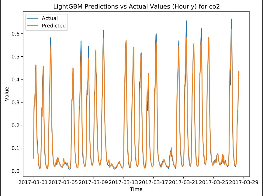
| CO2 | LightGBM | 0.0003834291266491532 | 0.0960325396742516 % |
| Humidity | SVR | 5.930342021103925e-05 | 0.01851282401967276 % |
| PM10 | XGBoost | 2.649203592035359e-05 | 0.041401718434739304 % |
| PM25 | XGBoost | 6.058677648190005e-05 | 0.03985426224063079 % |
| Temperature | SVR | 0.0002899542450183089 | 0.026371552642149455 % |
| VOC | SVR | 0.00043322552369807647 | 3.195298841037611 % |
The top three performing models for different pollutant values are:
| Feature | Best Performing Models |
|---|---|
| CO2 | LightGBM, RandomForest, XGBoost |
| Humidity | SVR, LightGBM, XGBoost |
| PM10 | LightGBM, RandomForest, XGBoost |
| PM2.5 | XGBoost, LightGBM, RandomForest |
| Temperature | SVR, RandomForest, LightGBM |
| VOC | SVR, LightGBM , RandomForest |
for example here is the prediction on CO2 values by LightGBM model
This project is licensed under the MIT License - see the LICENSE file for detail
