The goal of the Behavioual Cloning Project was to navigate a simulated vehicle around a test track by using a Convolutional Neural Network to predict steering angles.
My solution to this project consists of the following source code files that are needed to develop the model:
- train.py: Contains code for the training of a CNN using
- a CSV file of the steering angles, throttled image files from centre, left and right vehicle cameras. This program takes arguments to control the training of the model.
- nvidia.py: This contains the code implementing the model used to predict the steering angles. It is called NVIDIA as the model is based upon the research NVIDIA did for using deep learning to control a self driving car (see their Aug 2016 blog article End-to-End Deep Learning for Self-Driving Cars.
- datagen.py: Contains the code for my data generator class ImageGenerator() that implements the file selection, reading from disk and image augmentation of the training images.
- drive.py: The Udacity provided utility for loading the trained model and interfacing it with the Udacity Car Simulator. The final version is largely unmodified from that provided apart form setting the speed from 9 to 25.
Additional files of interest which are aviailable are the:
- logs/train_20190317-170803.log: A log of the runtime training session.
- trained/nvidia_20190317-170803.h5: the resultant model that successfully predicts steering angles for Track 1 of the car simulator. This can be downloaded and used with the Udacity car simulator to drive the vehicle around Track 1 with the drive.py program (ie
python drive.py trained/nvidia_20190317-170803.h5).
The model can be run to navigate the vehicle around the Udacity Car simulator Track 1 simply upon the following command:
python drive.py trained/nvidia_20190317-170803.h5
The development environment the model was developed in was an Ubuntu 18.04 host loaded with:
- Python 3.6.
- Tensorflow r1.13.1 compiled for GPU with NIVIDIA CUDA 10.0
- Keras 2.2.4 The model is saved in HDF5 format using h5py version 2.9.0
The final model selected is based upon the NVIDIA End-to-End Deep Learning for Self-Driving Cars research/demonstration paper.
My implementation of the model is in the source file nvidia.py has 5 Convolution Layers and 3 Fully Connected Layers. Additionally embedded in the model input layers apply pre-procesing to the RGB input images of dimensions 160 high x 320 wide :
- a colourspace conversion layer changing RGB color space to YUV (160,320)
- a normalisation layer to scale the images values in the range of [-1, 1];
- a cropping layer to crop the input images to a region interest of the road that excludes the Horizon and bonnet of the car.
A diagrammatic representation of the model architecture is shown below. This has been illustrated using NN-SVG.
I verified the architecture of the designed vs actual model implementation conducted with Tensorboard to view the graph. I utilised in training a Keras callback to Tensorboard, see train.py, to logging the training and validation loss as well as store a copy of the neural network architecture graph. This verification I found invaluable in the 'Traffic Signs Classifier' project where I used the resultant graph visualised in Tensorboard to identify I incorrectly implemented a layer due to a silly typo, hence I have made it standard practice to visualise the actual implementation vs desired deigned implementation.
Each training run also writes out a summary the model architecture as text See 20190317-130803.log lines 68-134 by using the Keras command model.summary().
The convolution layers reduce the cropped YUV image from 80x160@3 input to a 2x32@64 filter output with each layer progressively increasing in depth capturing different features.
The first three convolution layers use the same layout of:
- 5x5 filter sizes moving across the filter slices with a 2x2 stride
- Non linear ELU Activation Function
- 2x2 Max Pooling Layer
- Batch Normalizaion regularization function
The next two convolution layers use the same layout of:
- 3x3 filter sizes moving across the filter slices with a 1x1 stride
- Non linear ELU Activation Function
- Batch Normalizaion regularization function
The output of the convolution layer is flattened to a 1x4096 and fed into 3 x Fully Connected Layers. Again each layer progressively reduces the output from the flattened 4096 output of the convolution filter layer to a fully connected 128 > 64 > 16 > 1 single value decimal output for the steering angle.
I added to the model regularisation in the forms of Batch Normalisation and Dropout to aid the models ability to produce 'alternate representations', generalisation and reduce over fitting. My method of applying regularisation was to use "Batch Normalisation" in in the Convolution Layers after non-linear activation and Max Pooling, whilst in Fully Connected Layers. Dropout was set to a 50% keep rate. The dropout rate greatly affected the number or training iterations required going form a consistent 8 epochs to requiring 30+ epochs.
The model didn't need a lot of parameter tuning as the chosen optimised in the implementation was the Adam Optimiser . The main considerations were were the initial learning rate which was chosen to be 0.0002. This was established though several runs as higher values in the order of 1e-2 and 1e-3 would cause a high rate of drop in the loss, though there were clear periodic oscillation around a minima. Choosing a smaller learning rate in the order of 1e-4 meant mode epochs were required for the loss to decrease to an asymptote plateau, though the validation loss was more. The learning rate was easily changed through a command line parameter --learn_rate 0.0002 being passed to train.py I also included a callback to a learning rate scheduler to force the decrease of the learning rate by half to a limit of 1e-5 when there was no change in the loss. The feature of the Adam optimiser, Ternsorboard callback to view losses and the learning rate scheduler reduced the need to perform the number of runs to the the model parameters.
The training data utilised to train the model was the sample Udcaity data provided with the project that provided 8036 steering angles with camera views of centre, left and right camera. I augmented this data by recording additional data from the simulator by:
- Driving around the track in reverse recording an additional 4292 steering angles with camera views. The strategy behind driving reverse around the track was to provide additional steering angle data to aid in creating a balanced data set where there is not a bias to turning left or right.
- Short recovery driving session to record recovery angles where the car would drive off the track unless there was a steering correction input. This was done around several points on the track where there were different surface transitions on the edge (eg, road -> read-white chicane, road -> ripple strip, road -> lines, road -> dirt) where the steering angles for correction were established and then the recording for the recovery made. This added an additional 1259 steering angles with camera views.
Thus the data set used for training and validation totalled 13587 steering angles
Initial Models
My model development and training strategy was iterative. I initially built basic models like what was illustrated in the lectures like
- simple.py : A model where the cropped RGB images were flattened and fed into a Dense output layer
- lenet.py: A simple LeNet style model with 2 x Convolution followed by 2 x Fully Connected layers eith RELU activation.
These models formed the basis for developing the train.py training harness where the python library argparse was used to set default and enable variation in the training modes (eg dropout, early stopping, left right camera offset correction, multi=processing).
Data Generator
What was evident in these early stages of development was that my initial data generator based on a python loop with yeild() was inefficient as there was low GPU utilisation and training times per epoch were in the order of minutes for such a small data set. I profiled the GPU code with (NVIDIA Visual Profiler)[https://developer.nvidia.com/nvidia-visual-profiler] which showed that there were large pauses in the GPU operating the the code waiting on thread locks when the keras fit_generator() function was used with multiprocessing workers. My loop generator was decorated with an @threadsafe_generator() to synchronise access to the generator. Unfortunately it seems that the side effect was it stalled the worker threads from loading and preprocessing images from the disk.
I progressed to developing a new generator class called ImageGenerator(...) which extended the keras.util.Sequence. The Keras Sequence class is a utility class that can be used to guarantees each sample per epoch will only be trained once. My ImageGenrerator(Keras.util.Sequence) class also had these effect benefit of keeping the code clean and functionality encapsulated. All iamges are read from teh disk at runtime keeping the memory free and allowing an unlimited data size set to be used for training.
Early Results
The results of the simple models were a pleasent surprise. Initially the car would startonthe track and begin navigating, thought the car would not negotiate corners well and at times drive off the track even in straight sections. The steering was also erratic at times, seemingly fixating on a track feature. Adding dropout to the LeNet like model Fully Connected layers smoothed the steering significantly. It was clear that dropout generating the steering angel, though the vehicle would still drive off the track. My thoughts about this were that the model doesn't have the capacity to recognise the required features of the road and the road edges in order to steer appropriately nor to create 'redundant representations' to generalize the detection of the road.
Final Model
With the trail of though of having the need to create a higher-capcity model to learn more features, I progressed implementing 5 Convolutional Layer, 3 Fully connected layer network based upon the work done by NVIDIA. The number of filters per layer mimicked that presented in the End-to-End Deep Learning for Self-Driving Cars research paper, though my model differs in the size of the cropped input image being 80x320 instead of 66x200 as that being used in the NVIDIA's implementation. My process with developing the model went as follows:
- Get the vehicle driving around the track first with just the convolutional layers first, no regularisation.
- Add regularisation with Batch-Norm and Dropout and to generalise and prevent overfitting.
My implementation of the NVIDIA inspired model with Batch-Norm and Dropout was completely capable of driving around the track. There were sections where the network agent seemed to want to avoid shadows, though I came up with a strategy to combat this which is discussed in my next section "Mechanics of Training".
Of note, my image size is larger than that used in the NVIDIA model, there is highly likely to be an exceess in the number of parameters in my network that that required to navigate the one type of track. Essentially I really want the Convolution layers to recognise thread edges on the track and for the fully connected layers to set weights to create the steering inputs.
All of the source code used for training is detailed in train.py. As mentioned above, I used several sources of data:
- The original Udacity Provided Data.
- My recorded data set of traversing the track in the reverse direction.
- My recorded data set of Recovery Driving with steering inputs to re-center the vehicle on the track.
In the early stages of development, to facitlitate loading of the data I created a load_data() function that would glob the data directory (as specified with the --datadir argument) for the file driving_log.csv file that recorded the location of the file images as well as the throttle levels and steering angles. The data was stored in delimited CSV. The function load_data() performed the following functions:
- Loading the CSV data into a pandas data frame using appropriate addressable column names.
- Fixing file name paths of all of the files to the correct relative path.
- Smothing Steering Data with an exponential weighted moving filter (see DataFrame.ewm()) from the pandas library. The exception to this rule was the recovery data set there were only short consecutive recordings where I didn't the initial abrupt evasive angle smoothed out. Upon reflection, this step is probably not necessary with drop-out regularisation added in the fully connected layers as this will smooth out the steering as was seen in the early sates of the simple LeNet model when drop-out was added.
- Binning Steering Data by cutting and sorting the data into steering angle 'bins' based upon the steering angle in radians. The bins were fine grained by 0.1 radian around the majority 0 degree angle up to 0.5 radians. Coarser bins were 0.5 to 0.75 radians and 0.75 to 1 radians. Thus the complete list of bins were an array as such:
array([-1. , -0.75, -0.5 , -0.4 , -0.3 , -0.2 , -0.1 , -0. , 0.1 , 0.2 , 0.3 , 0.4 , 0.5 , 0.75, 1. ])The data in these bins were then labelled with a value by adding a column in the Pandas DataFrame called 'bins'. - Making Training and Validation Datasets by shuffling the smoothed combined data set and diving the pandas data frames into a Training Set (80% of the data) and Validation Set (20% of the data)
Data Class Imbalance
I took my learnings from the 'Traffic Sign Classifier Project' where there was a class imbalance for dominant sign classes. This is also try for the steering data in this project. The distribution of the majority of the steering angles on the Udacity data set was +ve directions to steer to the left and these are all near zero. The problem with this is that if the vehicle ned to perform a recovery maneuver to stop driving off the track, the weight activation of this angle is diminished by the majority values in the data. This is the exact opposite of what is needed. I devised a clever strategy to prevent he class imbalance by proposing that all data angled should be able to be drawn upon equally.
Data selected for a training batch is done by:
- grouping the training data into their bin label data angle.
- randomly bin selection of which steering angles will be a part of the batch.
- random sampling an steering angle and image from within a bin based upon the number of samples to be taken from each bin to fulfil the batch size.
This algorithm is implemented in my ImageGenerator(...). The data in the pandas data frame grouped with the private function __group_bins(df). These steering angle groups are then each sampled by a number of samples per groups calculated by:
samples_per_group = ceil(self.batch_sz / groups.ngroups)We then sample per steering bin this number of samples: is implemented using Pandas sample functions taking a random sample from each batch calculated by:
curr_batch = self._df_groups.apply(lambda grp: grp.sample(self._samples_per_group, replace=True)).sample(
            self.batch_sz)
As we are rounding up the number of samples to be taken per bin, the number of overall samples may be greater than the batch size. This is fine as we just re-randomly sample the samples to the batch size hence the final .sample( self.batch_sz) at the end. This code can be viewed in the getitem() function around line 84.
This technique works very well. Additionally left, right camera images are used in addition to the centre images and images are randomly flipped left and right providing an alternative representation. When left and right camera images are used, a correction to the steering of 0.2 radians is applied in the opposite direction of the cameras position. So for a left camera view, the left side of the road is closer than what the car should normally be, thus the steering input needs to be a right turn to keep the car in the center of the road as that would appear from the normal center camera view. The opposite is true for the right camera view, where the road is closer that the normal center view, thus a left steering input needs to be applied to keep the car in the center.. The number of batches per epochs with this technique is somewhat arbitrary. I determined by the total number of lines steering data, divided by the batch size, though in reality it could be larger number that would probably result in less epochs to get a very much similar result.
Image Augmentation
This took a couple of goes to get this what I wanted. Data augmentation is highly desirable as the larger turning angles have a significant smaller number of data sets in the order of tens whilst those steering angles within +/-0.2 radians are in the order of thousands. An example of the training distribution of the steering angles in the bins is as follows:
| 'bin' | Samples |
|---|---|
| (-1.001, -0.75] | 170 |
| (-0.75, -0.5] | 162 |
| (-0.5, -0.4] | 97 |
| (-0.4, -0.3] | 142 |
| (-0.3, -0.2] | 366 |
| (-0.2, -0.1] | 605 |
| (-0.1, -0.0] | 2966 |
| (-0.0, 0.1] | 4883 |
| (0.1, 0.2] | 1021 |
| (0.2, 0.3] | 338 |
| (0.3, 0.4] | 53 |
| (0.4, 0.5] | 16 |
| (0.5, 0.75] | 11 |
| (0.75, 1.0] | 36 |
To aid the generalization of the model it is desirable to augment the inmage data to vary what the network 'sees' in order to generalize the problem space and enable the network to cope with un-seen/un-expected variations in the data it is presented with.
With this in mind I used the Python image augmentation library imgaug by Alexander Jung. This is a wrapper library for skimage and OpenCV libraries to perform image augmentation. Variations such as noise, perspective transforms, shifts and crops can be added sequentially and randomly to the image. I initially setup in my data generator to randomly select up to 3 augmentations from 9. This worked, though at times produced a not so smooth result. I did change my approach by reflect upon the essential goal of the network. The car is already on the simulator trackm it just needs to not drive off the track. I want the convolution layers in my network to learn the edges the track. Whith this condition in mind, ther are only two augmentations I decided I needed to make to the imgaes to the network more robust:
- Color shading (hue) variations - by varying the hue of the images by +/-30%. I don't really want the network to lean about colors, I actually want the network to learn about edges of the track. Thus if I reandomly vary the color/hue in the images, I lessen the importance of the colors of the road and the scene to be learnt.
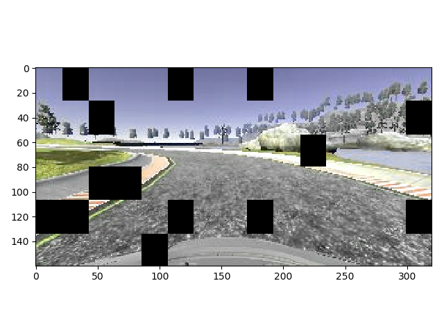
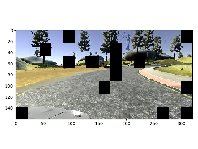
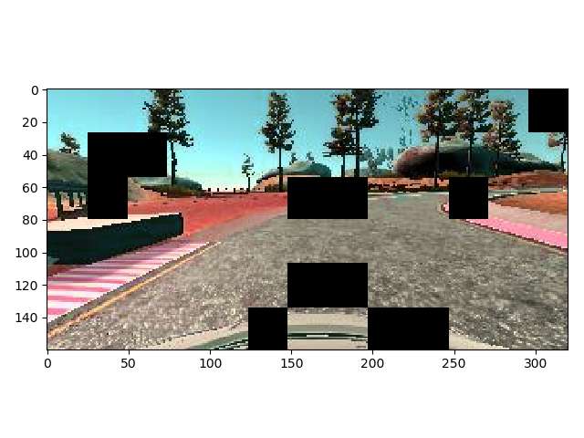
- Missing features - by adding the the image Coarse Dropout to the images. The track in the simulator has sections where the road is partially shadowed. In essence there is missing data/features that are less likely to be picked up in training the network in those regions. There is usually another edge of the road or some other feature such as as a line or un-shadowed road ahead which can be used to navigate from. Why not force this in the learning of the data. A real world illustration of this is driving on the road. If there is a car in front of you and there is also person standing on the road edge waiting to cross, though slightly more difficult, our brain still can work out where the edge of the road is from a lesser set of features. Effectively the car and the person obscuring a good view of the road is just noise. Using this princinple, I introduced coarse dropout in my image augmentation to make the network more robust to partial and obscured features in the road like shadows and noise like road textures.
The image augmenters are setup in the ImageGenerator() class with the function __init_image_augmenter() (see lines 25-29 of the source code). All images are subject to augmentation of both Hue variation, there are no original images used for training. Similarly there is a 50% chance that any image in a batch can be flipped.
The same augmentations that are applied to the training set are applied to the validation data set. The same generator is also used as I want the validation loss values against the same agumentations and image selections as that on the training data set. Though still acceptable, I don't want to artificially bias the validation result by giving raw clean image data.
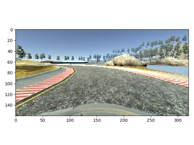
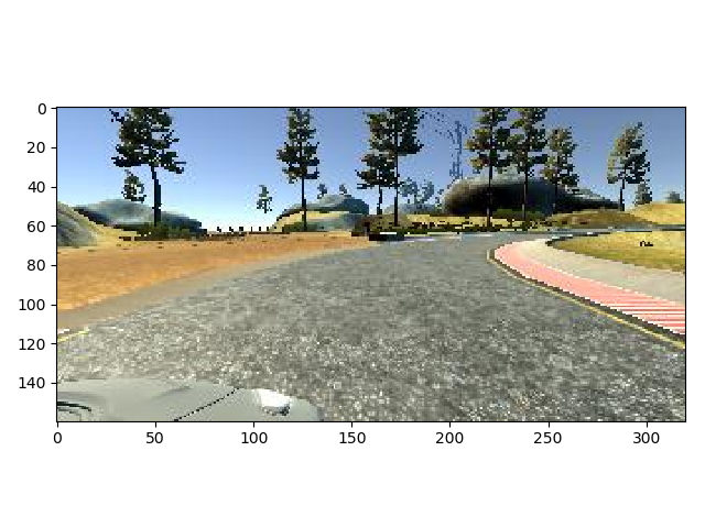
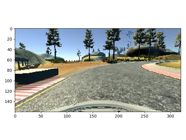
Here are three examples of three image augmentations taken at runtime from my ImageGenerator class. The Original image is on the LEFT and the Augmented image is on the RIGHT.
1 Moderate Hue changes, Coarse Dropout affecting the visability of the near left line.
2 Slight Hue changes, Coarse Dropout acting as slight road noise. Of note this image is the right side camera. Additionally of note is that this is an image from the reverse direction around the track, or, has been flipped left/right around the vertical axis.
3 Strong Hue changes, Coarse Dropout affecting straight ahead and turn visability. Also of note is that this is an image from the reverse direction around the track, or, has been flipped left/right around the vertical axis.
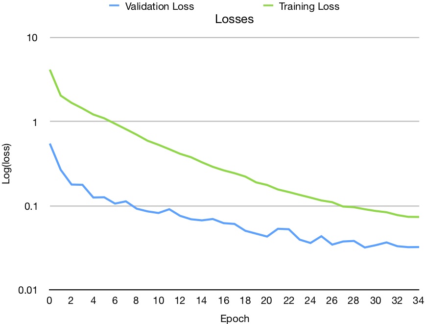
Here I present the training losses for the final model in the repository nvidia_20190317-170803.h5 The loss values are presented on a log scale. There were 34 epochs as the validation loss values started to increase again and Keras saved the model with the lowest loss and terminated the run after 5 consecutive, though small, increases in the loss. Though built in as a facility of the code, I did not have learning rate scheduling turned on to force the reduction in the learning rate for the final solution.
I have uploaded my result of running on Track 1 to YouTube. The frame rate is set top 48fps to shorten the viewing time of the car travelling around the track.
Please click on the image below to view:
I am happy with my result. I can quickly (about 16 seconds per epoch) and easily train my network and reliably get a result of a vehicle to drive around the track at 25 to 30mph. I have learnt a lot in this project and I especially like the ease in which the Keras API offers to quickley implement models as well the integration of callbacks such as Early Stopping, Learning Rate Scheduling (to force a reduction in the learning rate) as well as Tensorboard. What I am interested in exploring in the project further is to get the car in the Udacity simulator travelling as far as possible around Track 2 without ever being Trained on Track 1 data.

