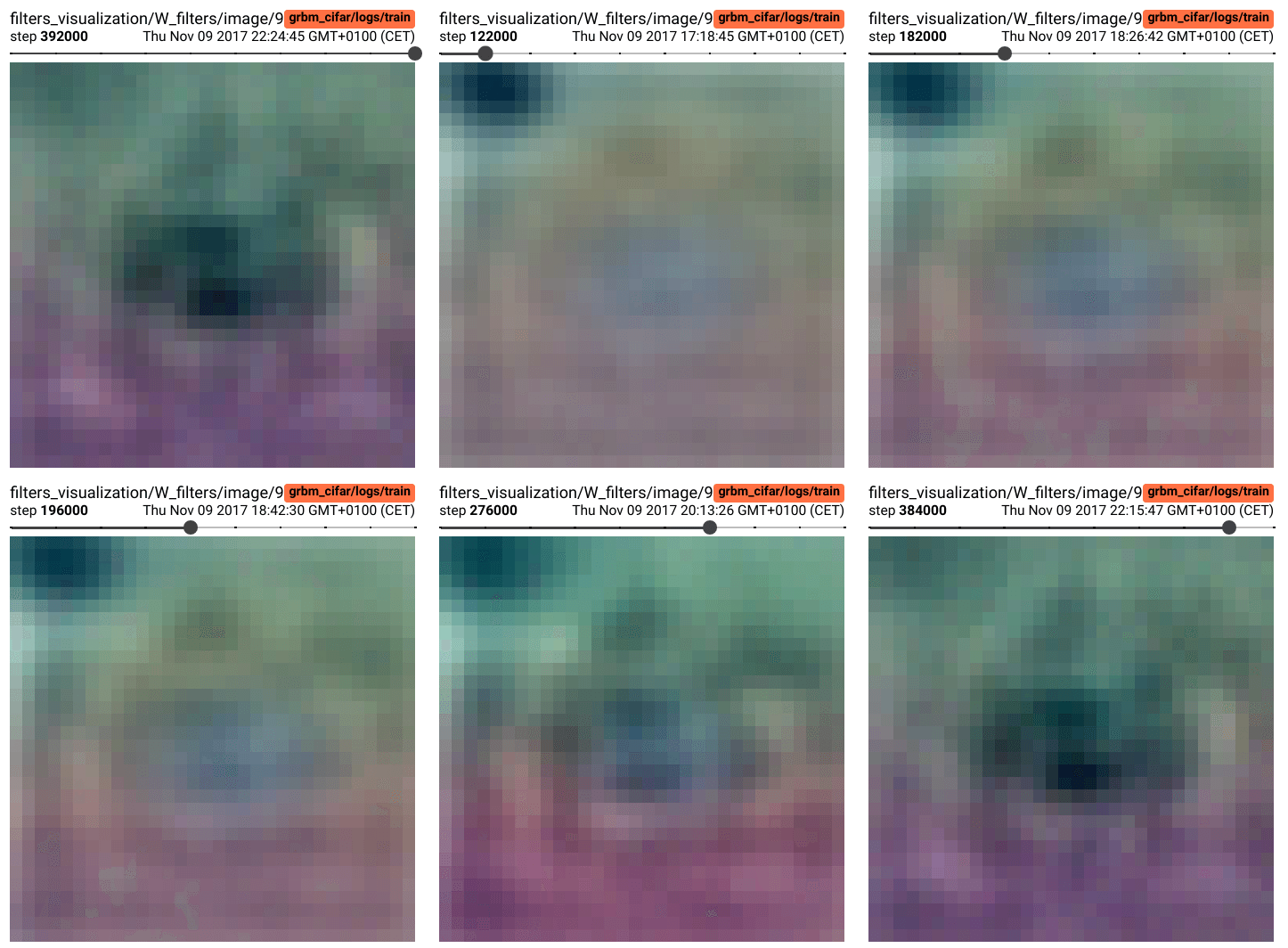
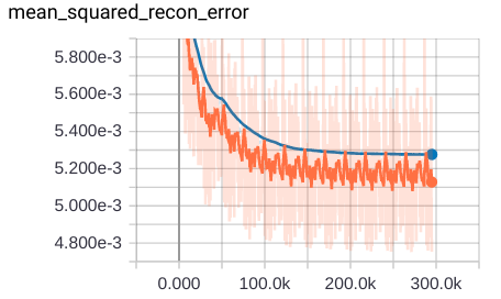
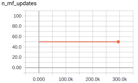
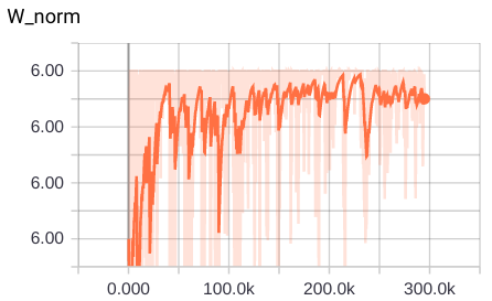
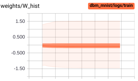
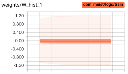
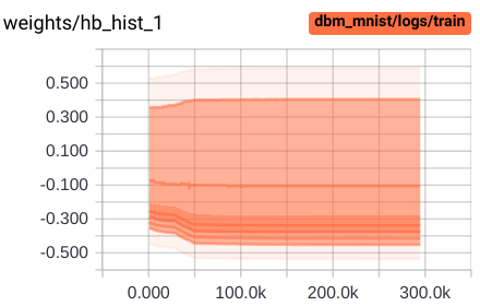
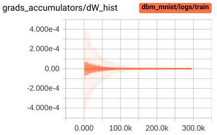
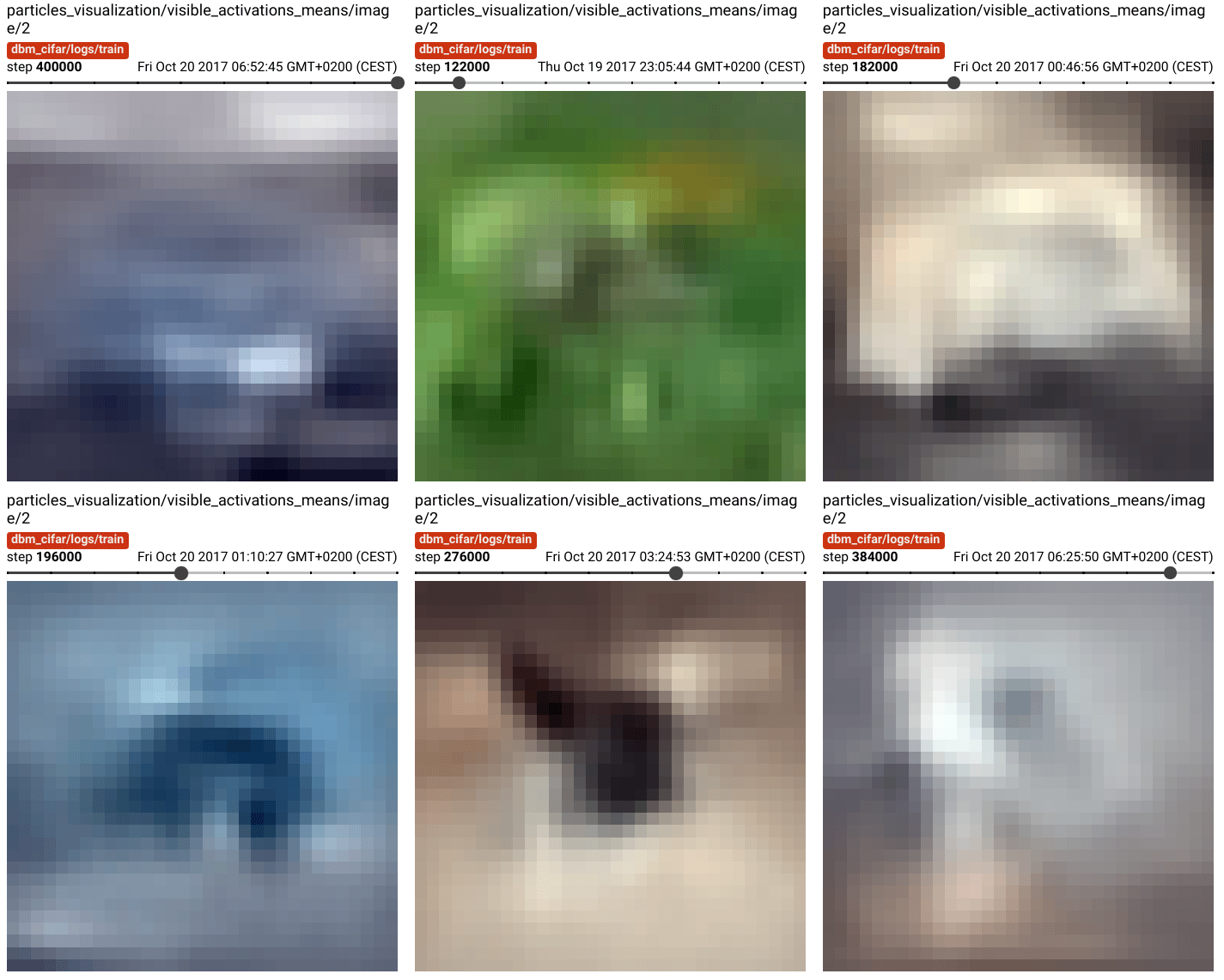
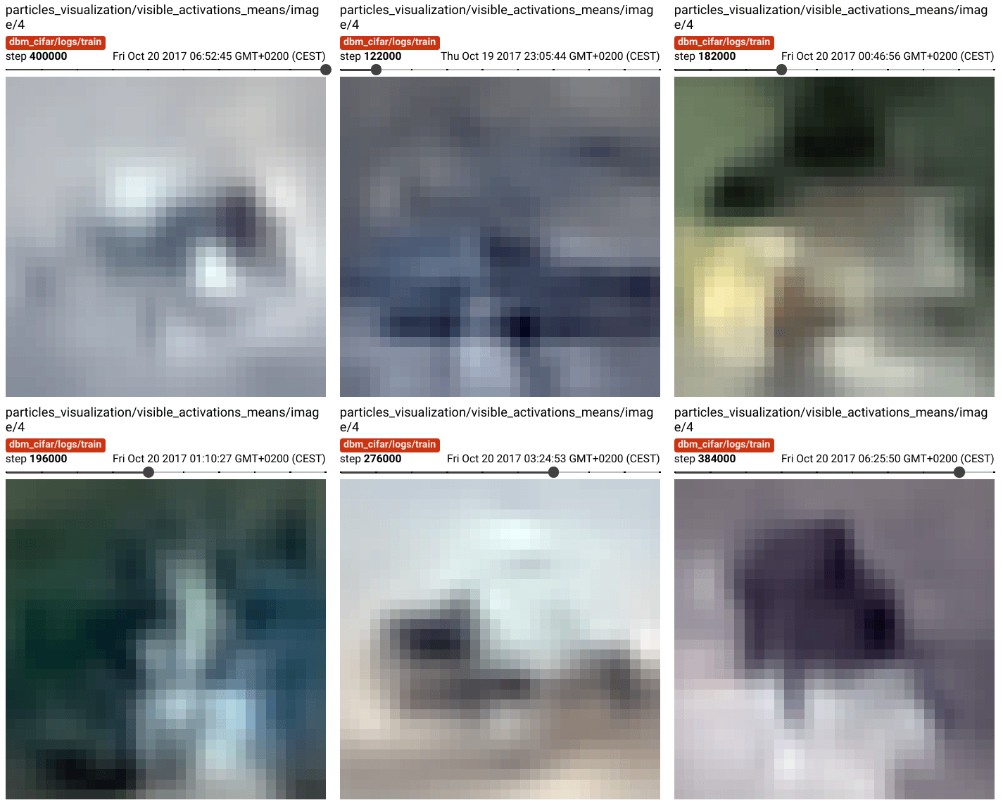
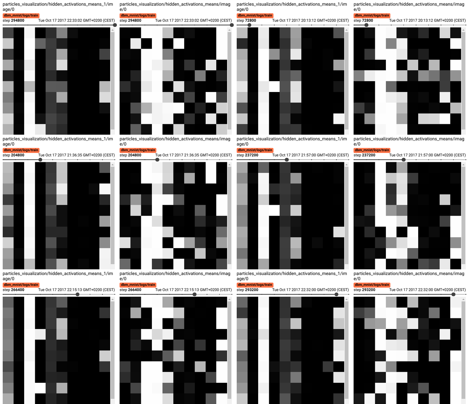
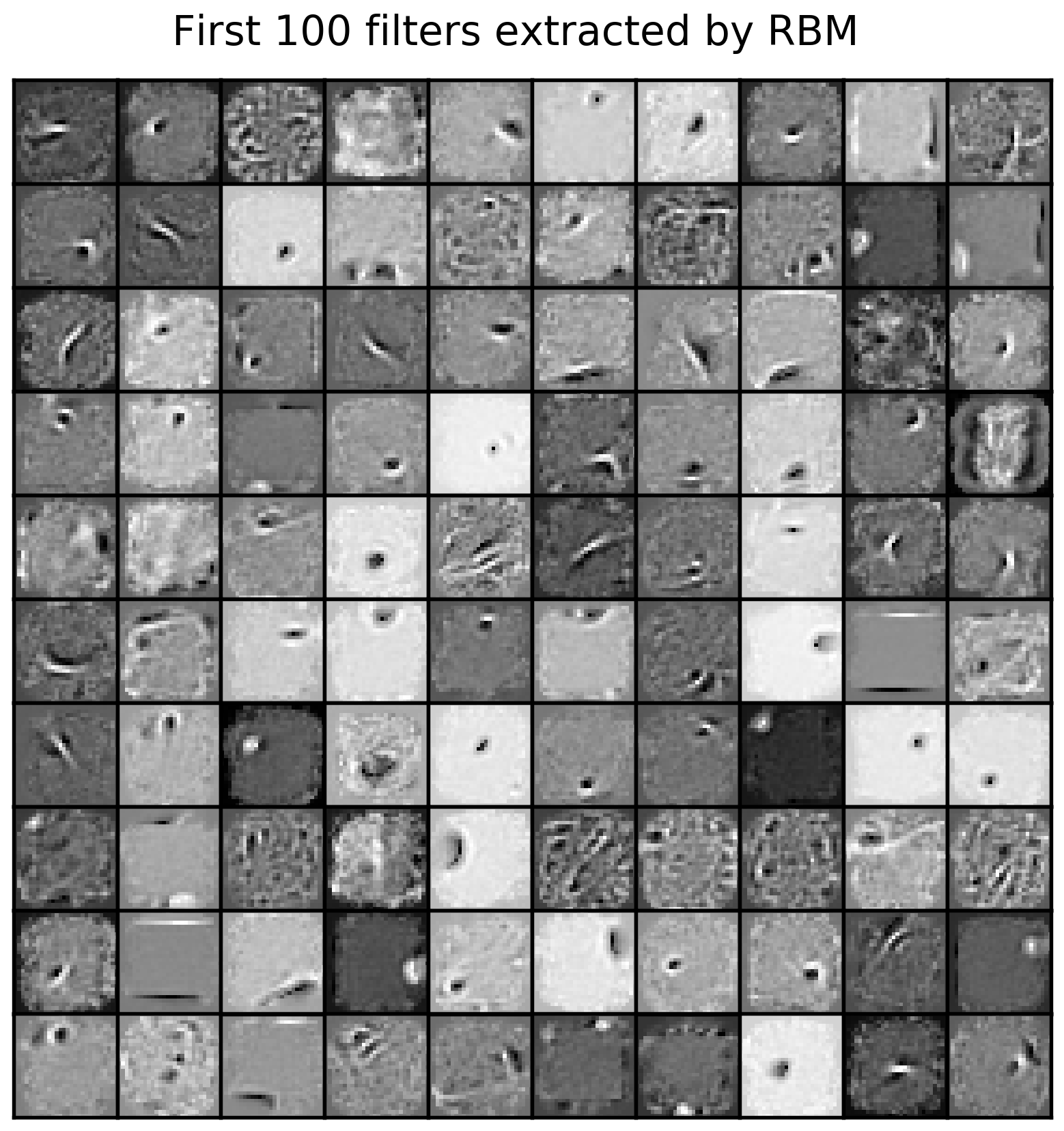
This repository implements generic and flexible RBM and DBM models with lots of features and reproduces some experiments from "Deep boltzmann machines" [1], "Learning with hierarchical-deep models" [2], "Learning multiple layers of features from tiny images" [3], and some others.
- What's Implemented
- Examples
- Download models and stuff
- TeX notes
- How to install
- Possible future work
- Contributing
- References
- [computational graph]
- k-step Contrastive Divergence;
- whether to sample or use probabilities for visible and hidden units;
- variable learning rate, momentum and number of Gibbs steps per weight update;
- regularization: L2 weight decay, dropout, sparsity targets;
- different types of stochastic layers and RBMs: implement new type of stochastic units or create new RBM from existing types of units;
- predefined stochastic layers: Bernoulli, Multinomial, Gaussian;
- predefined RBMs: Bernoulli-Bernoulli, Bernoulli-Multinomial, Gaussian-Bernoulli;
- initialize weights randomly, from
np.ndarray-s or from another RBM; - can be modified for greedy layer-wise pretraining of DBM (see notes or [1] for details);
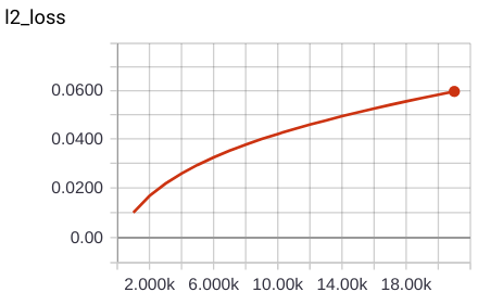
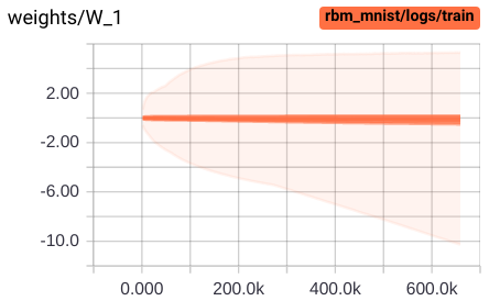
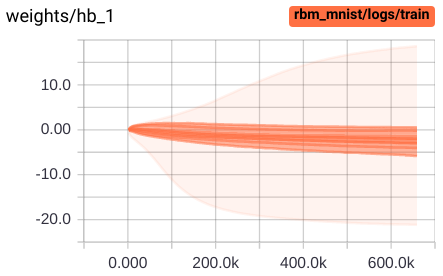
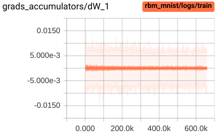
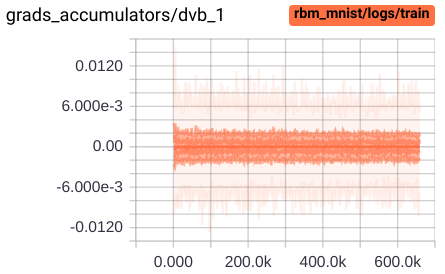
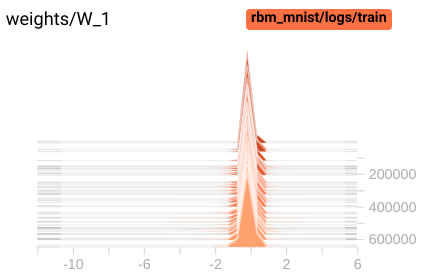
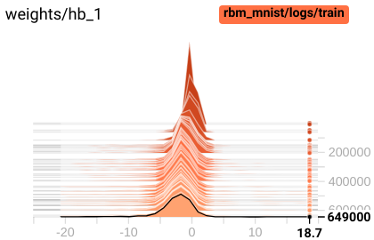
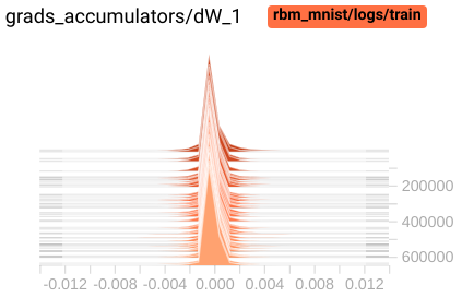
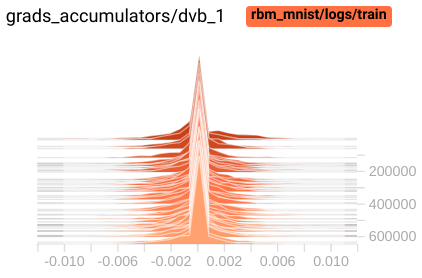
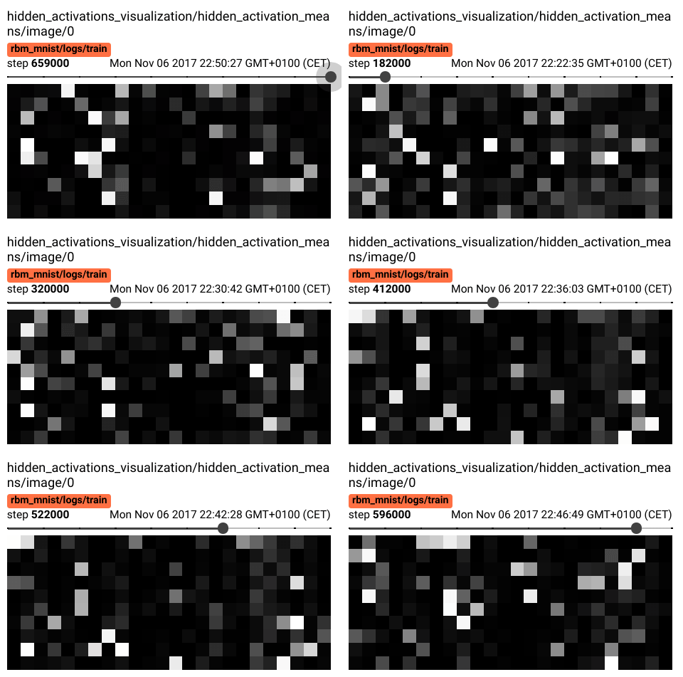
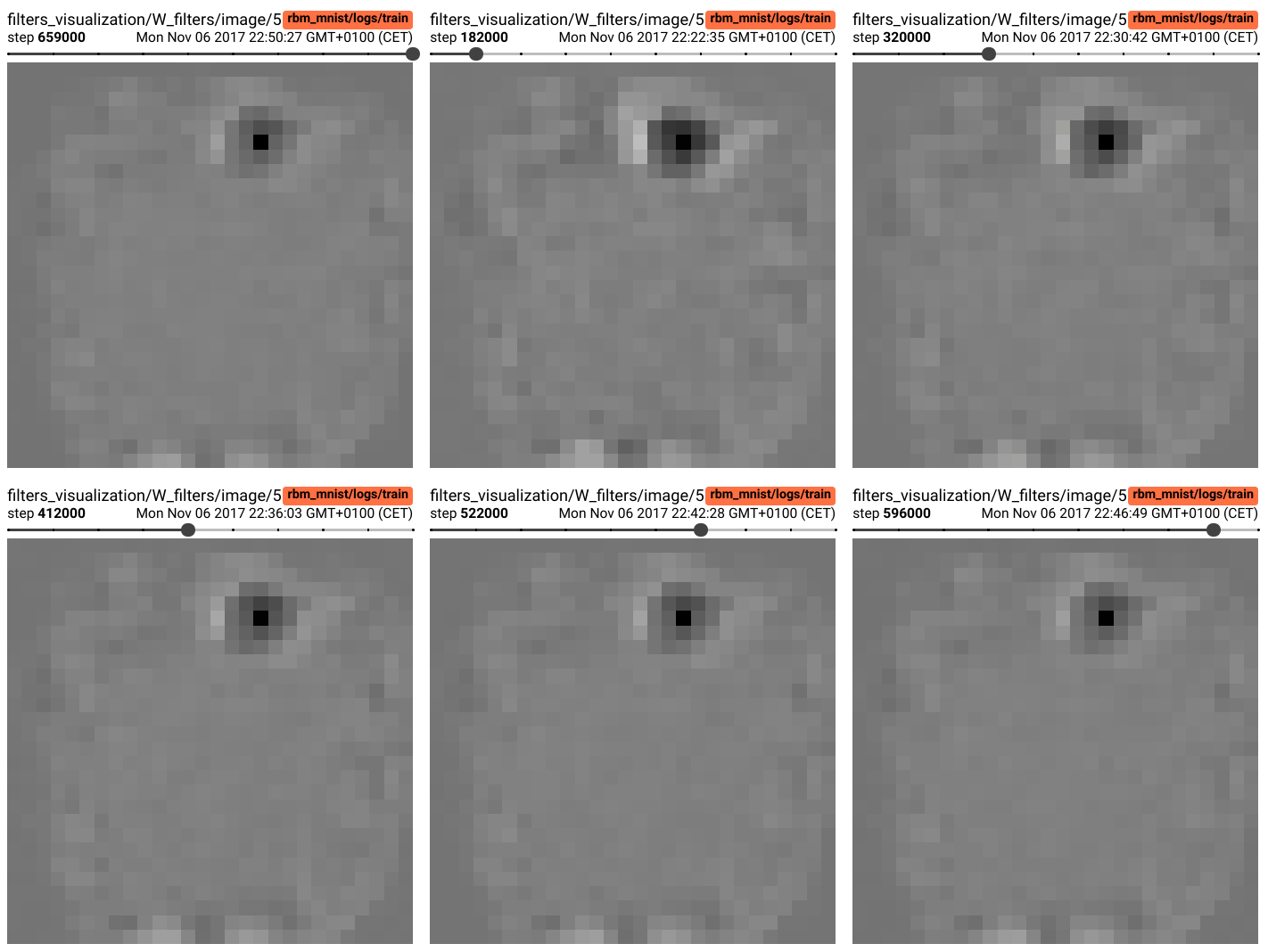
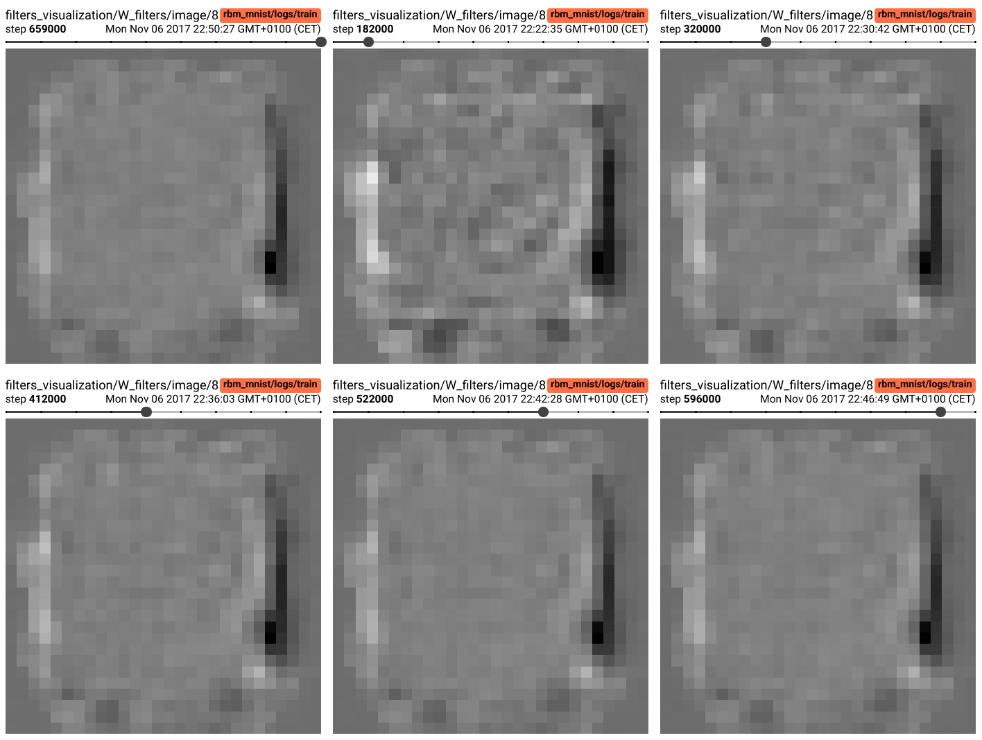
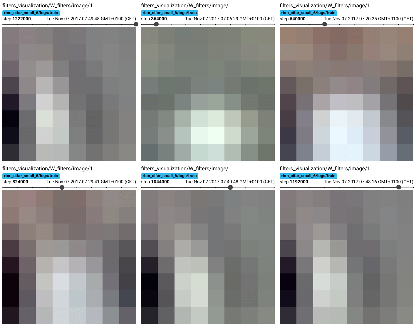
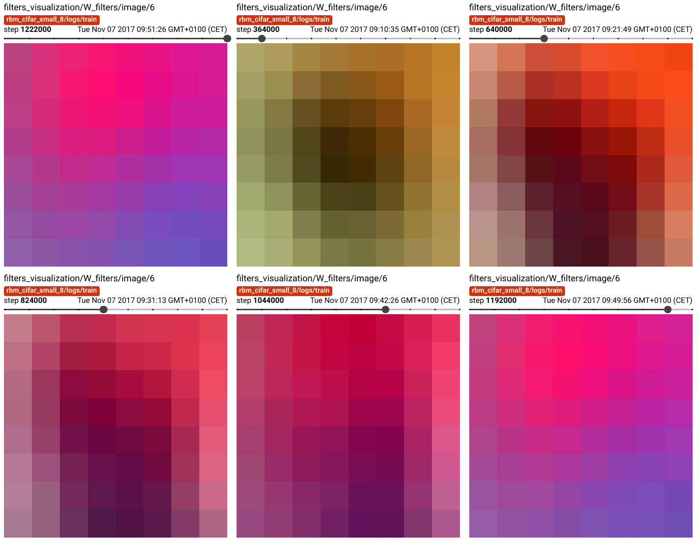
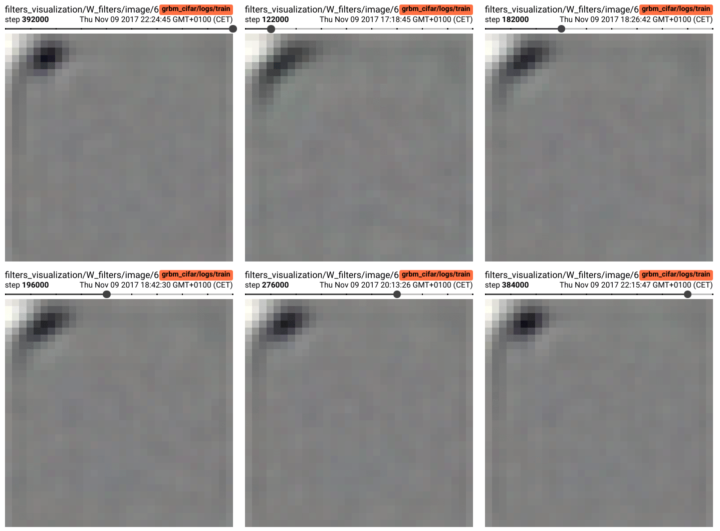
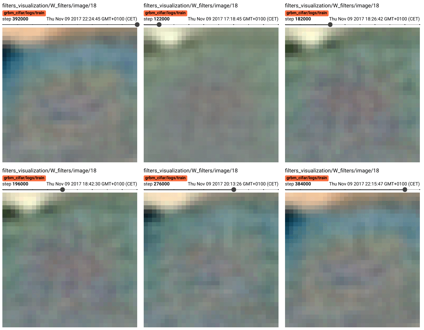
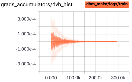
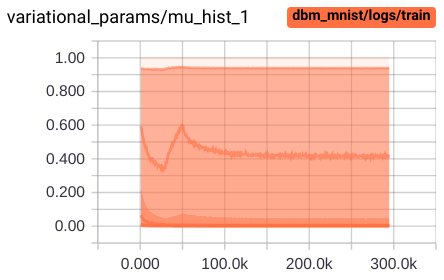
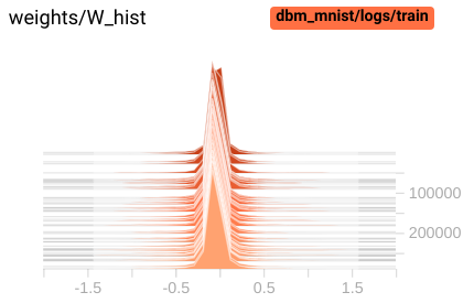
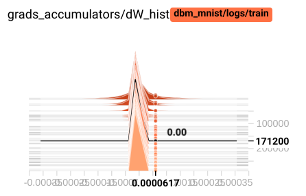
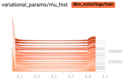
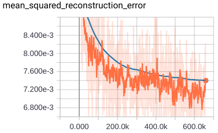
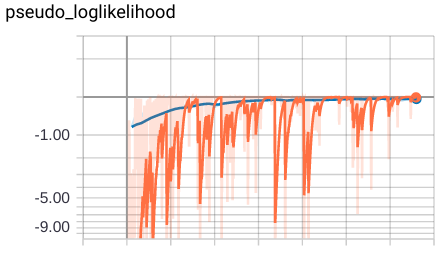
- visualizations in Tensorboard (hover images for details) and more:
- [computational graph]
- EM-like learning algorithm based on PCD and mean-field variational inference [1];
- arbitrary number of layers of any types;
- initialize from greedy layer-wise pretrained RBMs (no random initialization for now);
- whether to sample or use probabilities for visible and hidden units;
- variable learning rate, momentum and number of Gibbs steps per weight update;
- regularization: L2 weight decay, maxnorm, sparsity targets;
- estimate partition function using Annealed Importance Sampling [1];
- estimate variational lower-bound (ELBO) using logẐ (currently only for 2-layer binary BM);
- generate samples after training;
- initialize negative particles (visible and hidden in all layers) from data;
DBMclass can be used also for training RBM and its features: more powerful learning algorithm, estimating logẐ and ELBO, generating samples after training;- visualizations in Tensorboard (hover images for details) and more:
- easy to use with
sklearn-like interface; - easy to load and save models;
- easy to reproduce (
random_seedmake reproducible both TensorFlow and numpy operations inside the model); - all models support any precision (tested
float32andfloat64); - configure metrics to display during learning (which ones, frequency, format etc.);
- easy to resume training (note that changing parameters other than placeholders or python-level parameters (such as
batch_size,learning_rate,momentum,sample_v_statesetc.) betweenfitcalls have no effect as this would require altering the computation graph, which is not yet supported; however, one can build model with new desired TF graph, and initialize weights and biases from old model by usinginit_frommethod); - visualization: apart from TensorBoard, there also plenty of python routines to display images, learned filters, confusion matrices etc and more.
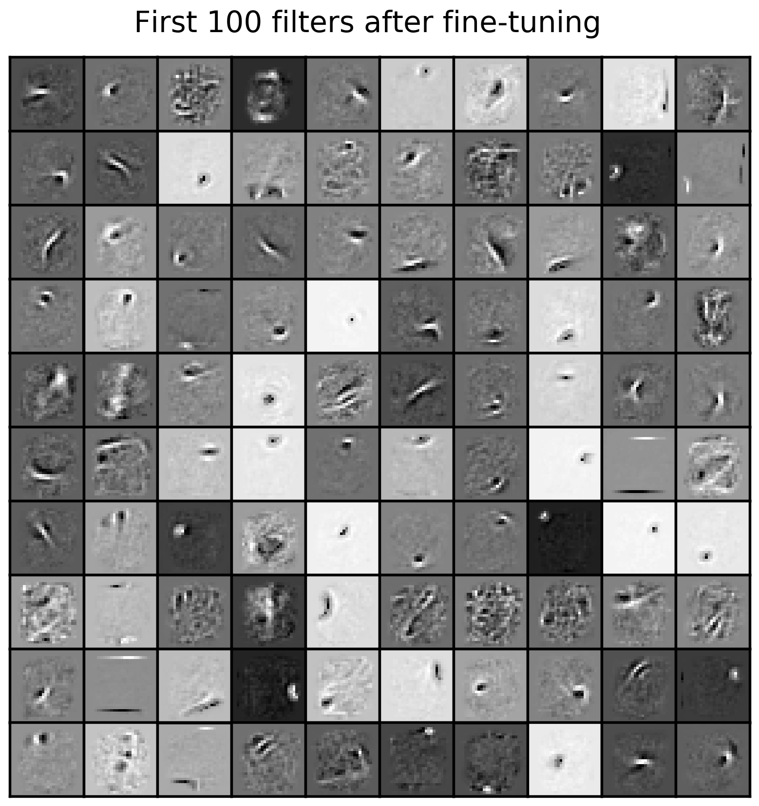
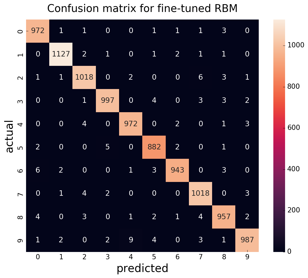
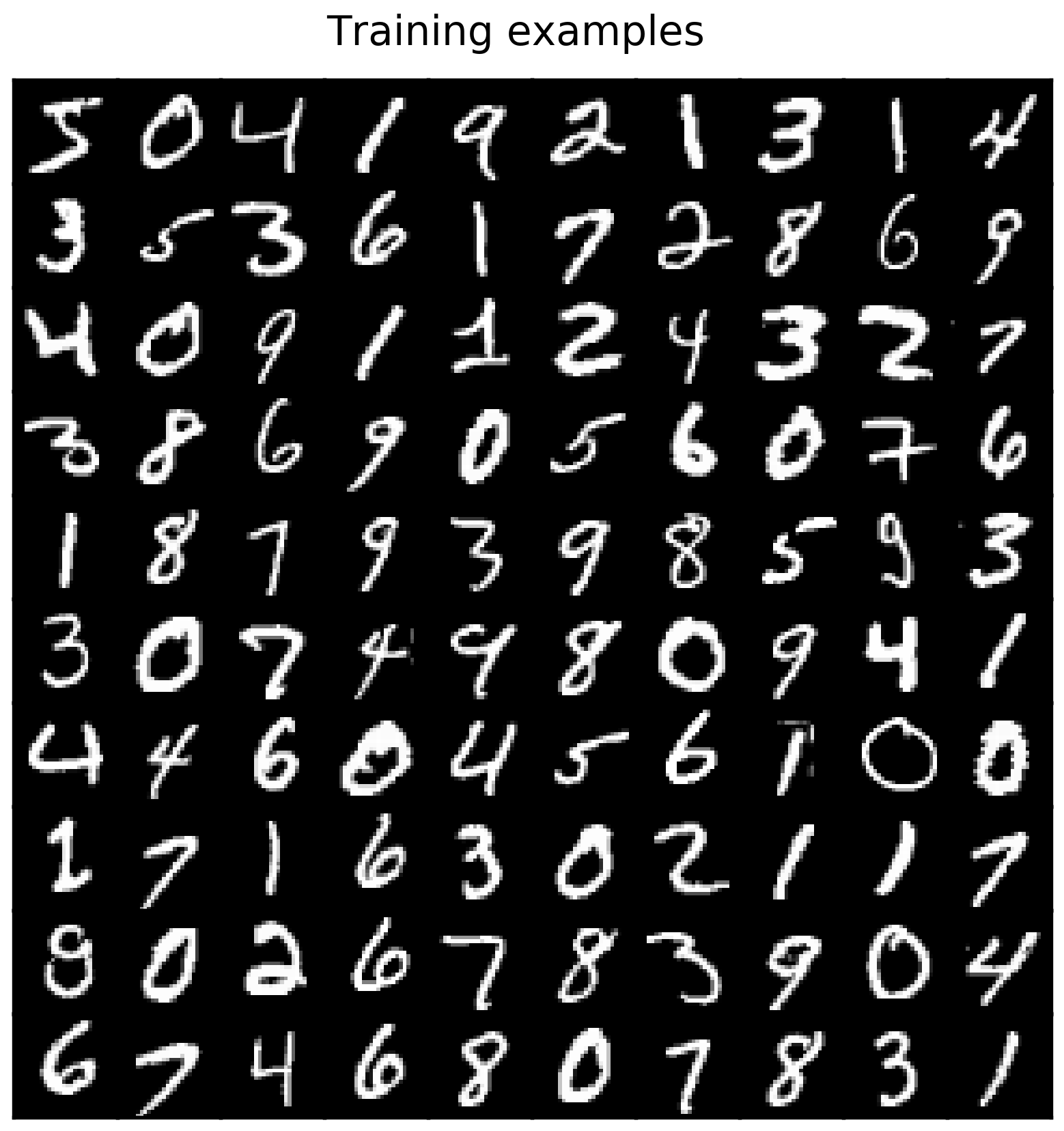
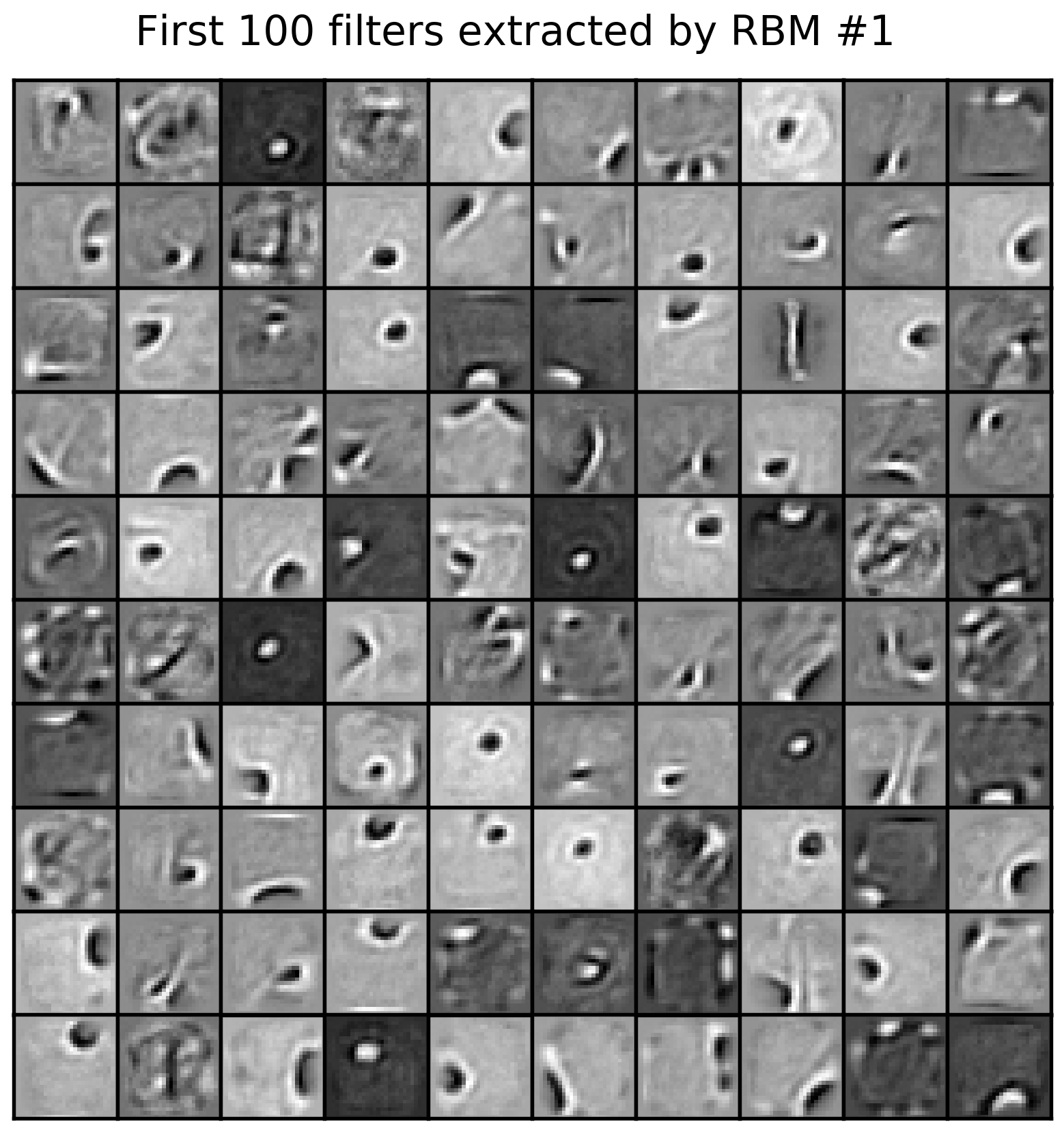
Train Bernoulli RBM with 1024 hidden units on MNIST dataset and use it for classification.
algorithm |
test error, % |
|---|---|
| RBM features + k-NN | 2.88 |
| RBM features + Logistic Regression | 1.83 |
| RBM features + SVM | 1.80 |
| RBM + discriminative fine-tuning | 1.27 |
Another simple experiment illustrates main idea of one-shot learning approach proposed in [2]: to train generative neural network (RBM or DBM) on large corpus of unlabeled data and after that to fine-tune model only on limited amount of labeled data. Of course, in [2] they do much more complex things than simply pre-training RBM or DBM, but the difference is already noticeable:
| number of labeled data pairs (train + val) | RBM + fine-tuning | random initialization | gain |
|---|---|---|---|
| 60k (55k + 5k) | 98.73% | 98.20% | +0.53% |
| 10k (9k + 1k) | 97.27% | 94.73% | +2.54% |
| 1k (900 + 100) | 93.65% | 88.71% | +4.94% |
| 100 (90 + 10) | 81.70% | 76.02% | +5.68% |
How to reproduce the this table see here. In these experiments only RBM was tuned to have high pseudo log-likelihood on a held-out validation set. Even better results can be obtained if one will tune MLP and other classifiers.
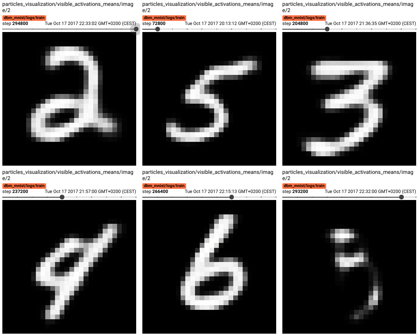
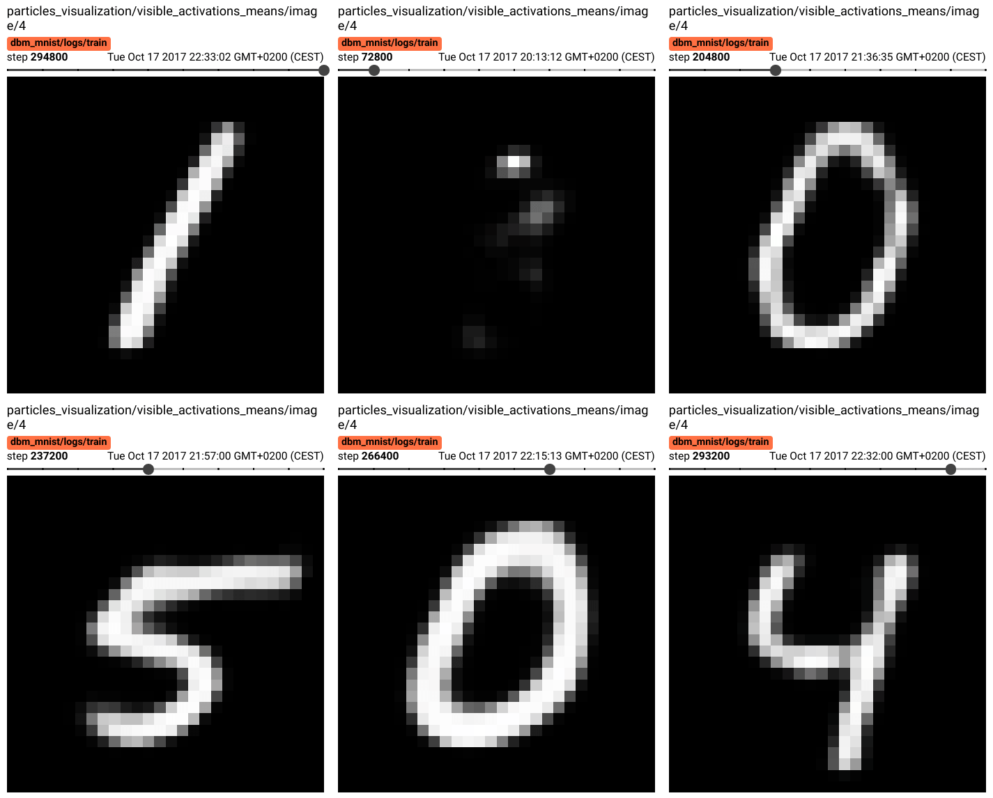
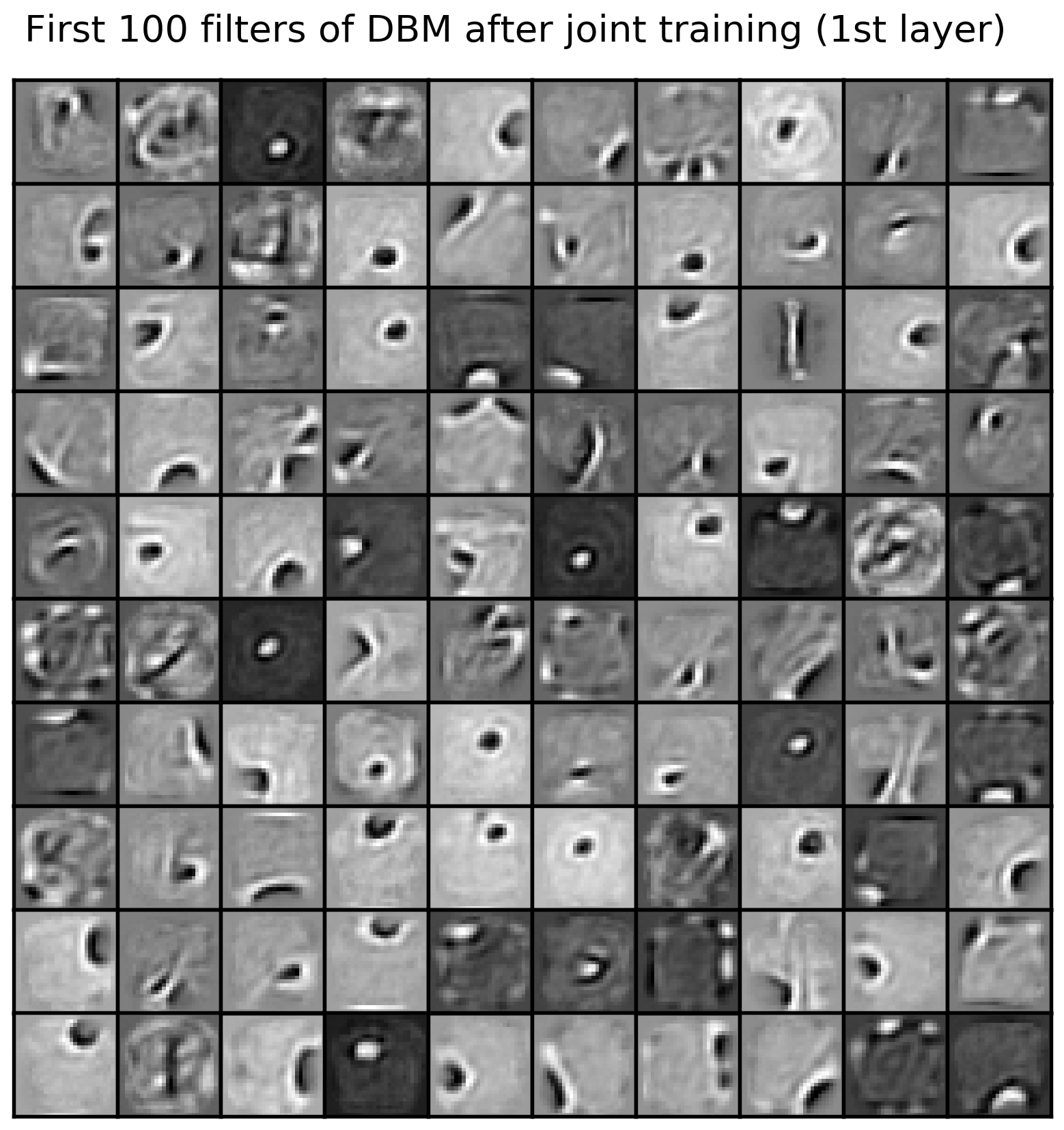
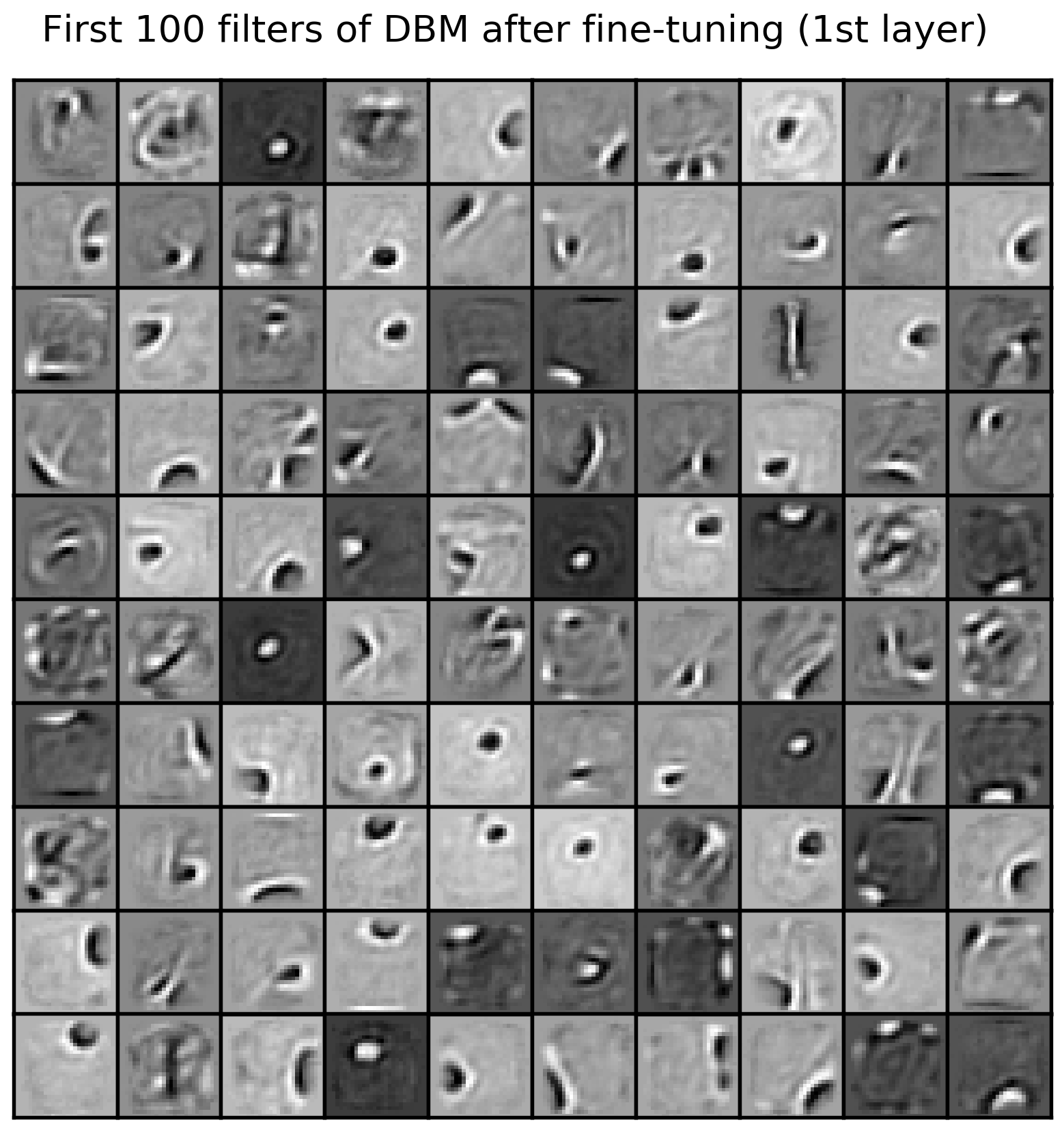
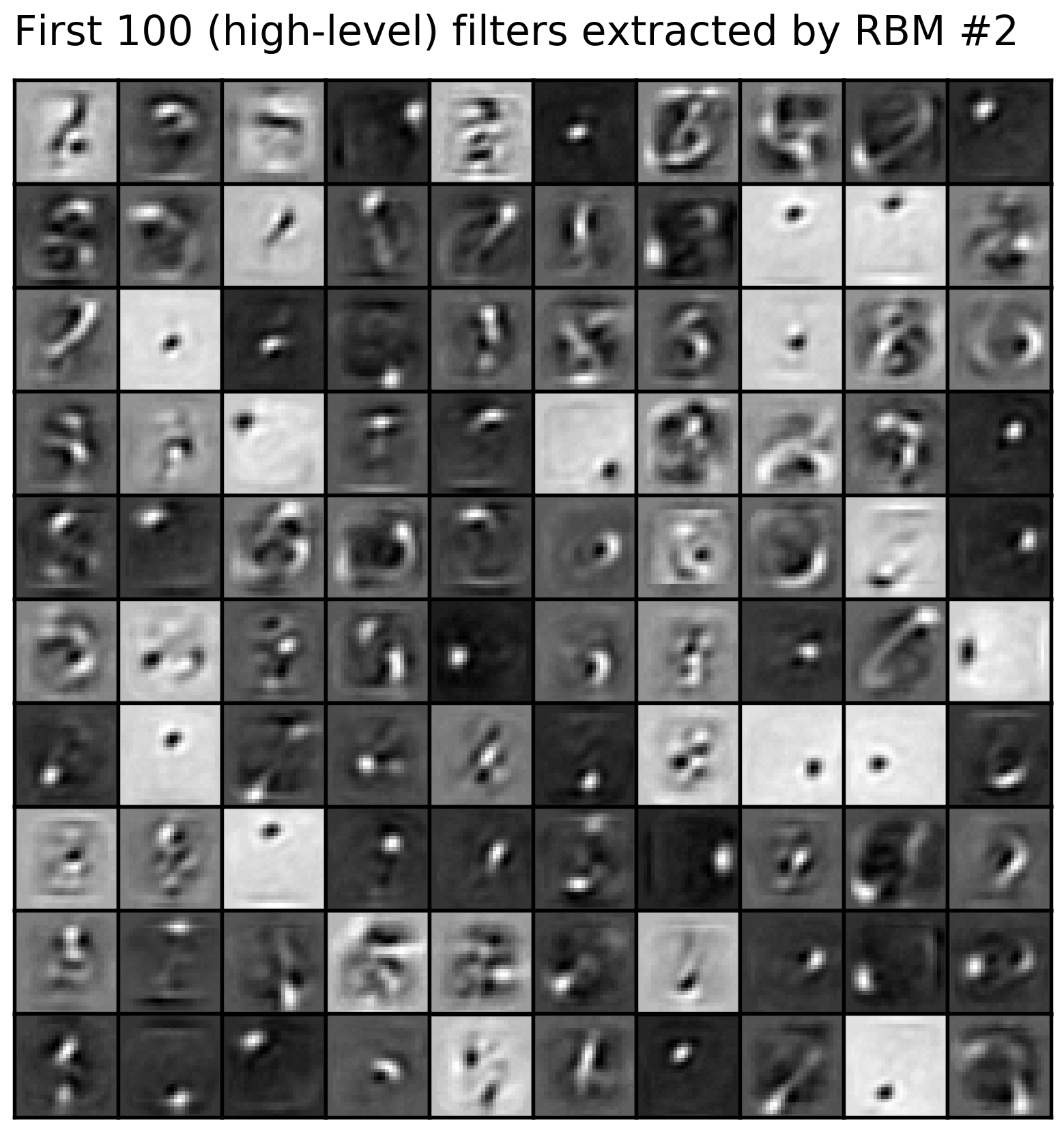
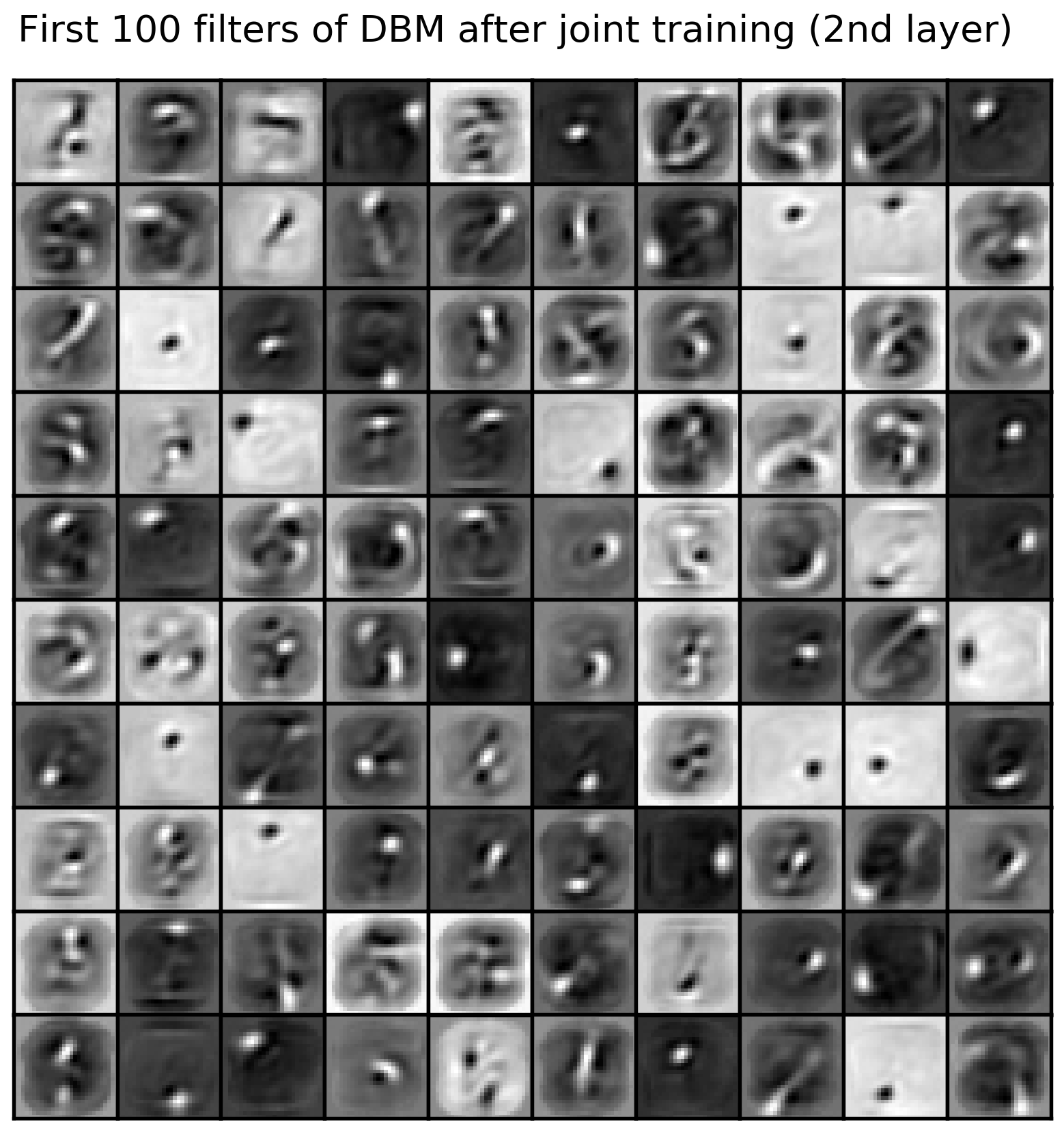
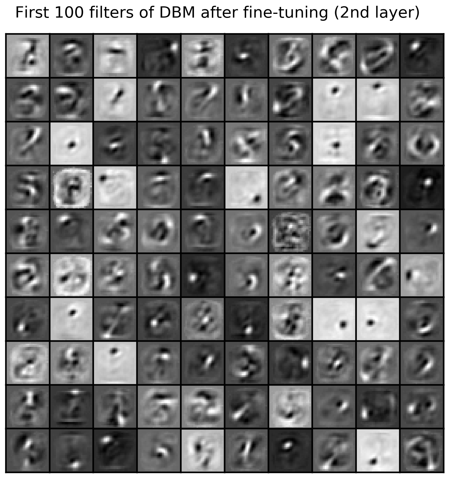
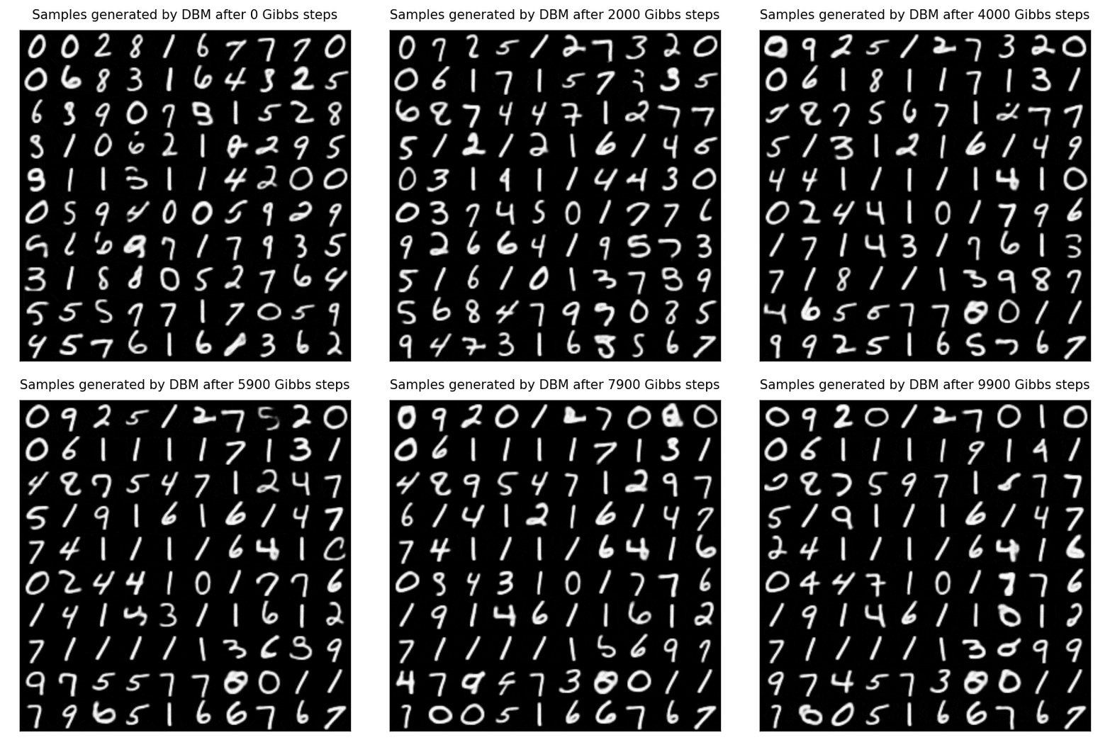
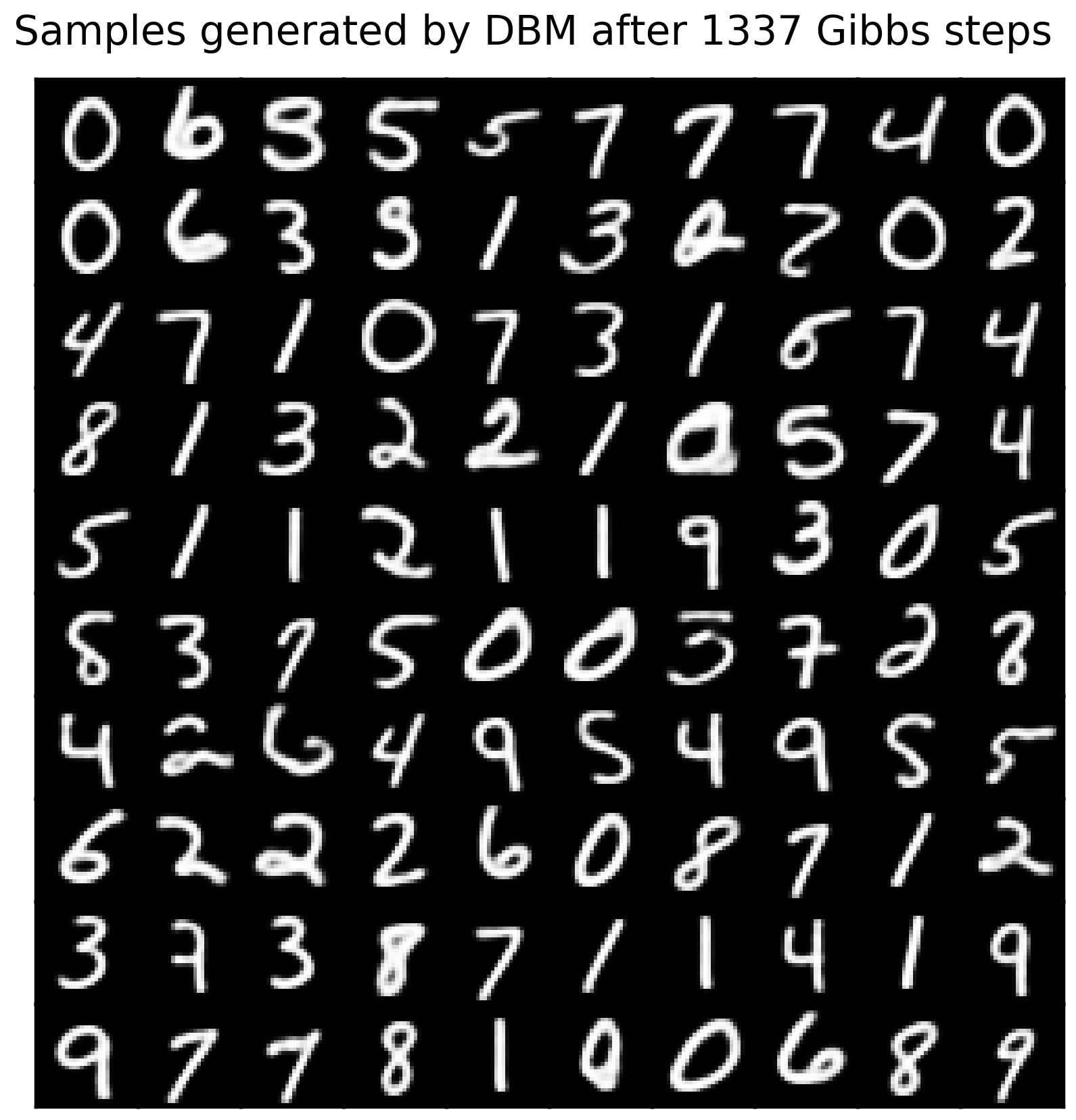
Train 784-512-1024 Bernoulli DBM on MNIST dataset with pre-training and:
- use it for classification;
- generate samples after training;
- estimate partition function using AIS and average ELBO on the test set.
| algorithm | # intermediate distributions | proposal (p0) | logẐ | log(Ẑ ± σZ) | avg. test ELBO |
|---|---|---|---|---|---|
| [1] | 20'000 | base-rate? [5] | 356.18 | 356.06, 356.29 | -84.62 |
| this example | 200'000 | uniform | 1040.39 | 1040.18, 1040.58 | -86.37 |
| this example | 20'000 | uniform | 1040.58 | 1039.93, 1041.03 | -86.59 |
Couple of nats could have been lost because of single-precision.
| number of labeled data pairs (train + val) | DBM + fine-tuning | random initialization | gain |
|---|---|---|---|
| 60k (55k + 5k) | 98.68% | 98.28% | +0.40% |
| 10k (9k + 1k) | 97.11% | 94.50% | +2.61% |
| 1k (900 + 100) | 93.54% | 89.14% | +4.40% |
| 100 (90 + 10) | 83.79% | 76.24% | +7.55% |
How to reproduce the this table see here.
Again, MLP is not tuned.
Performance on full training set is slightly worse compared to RBM because of harder optimization problem + possible vanishing gradients. Also because the optimization problem is harder, the gain when not much datapoints are used is typically larger.
Large number of parameters is one of the most crucial reasons why one-shot learning is not (so) successful by utilizing deep learning only. Instead, it is much better to combine deep learning and hierarchical Bayesian modeling by putting HDP prior over units from top-most hidden layer as in [2].
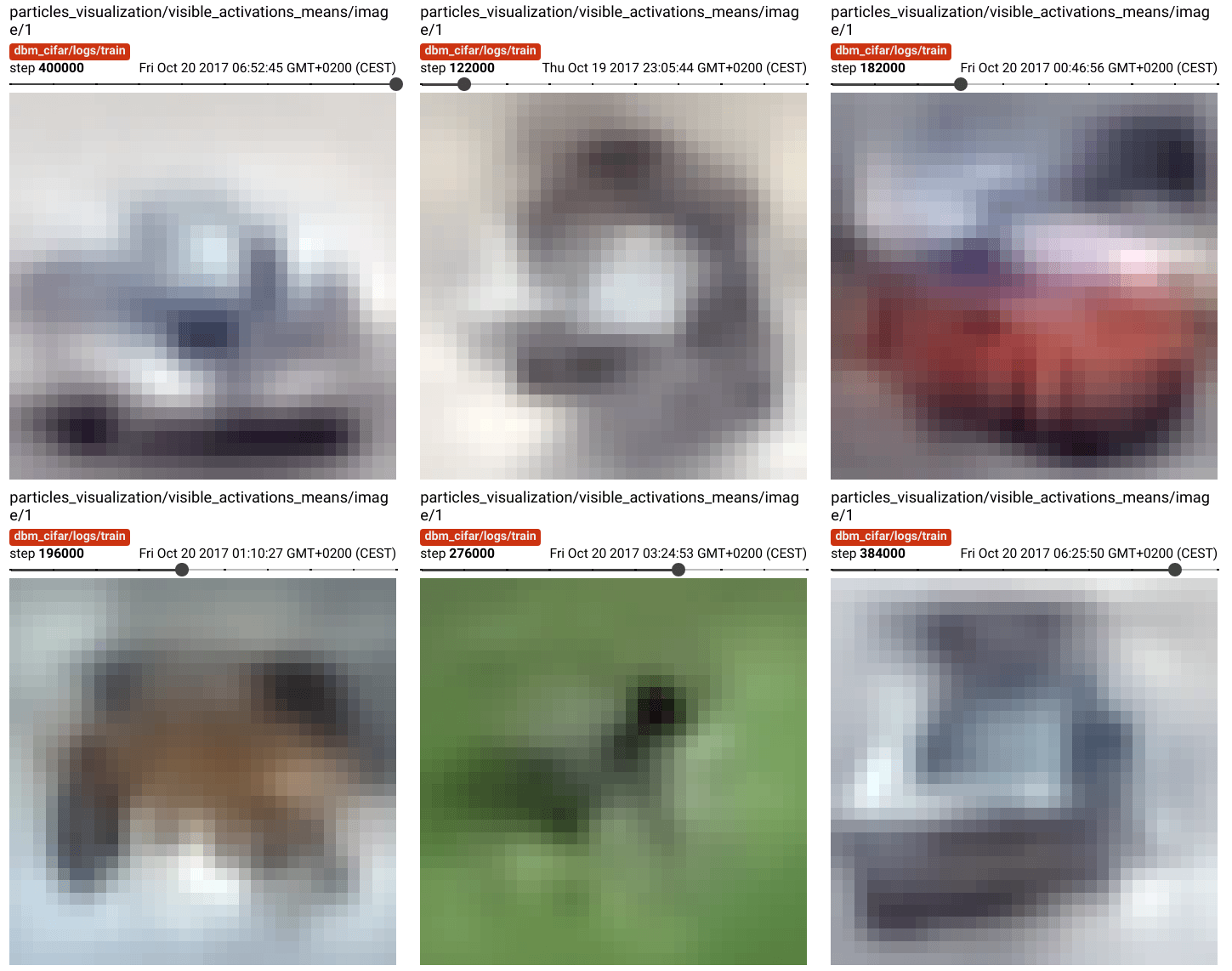
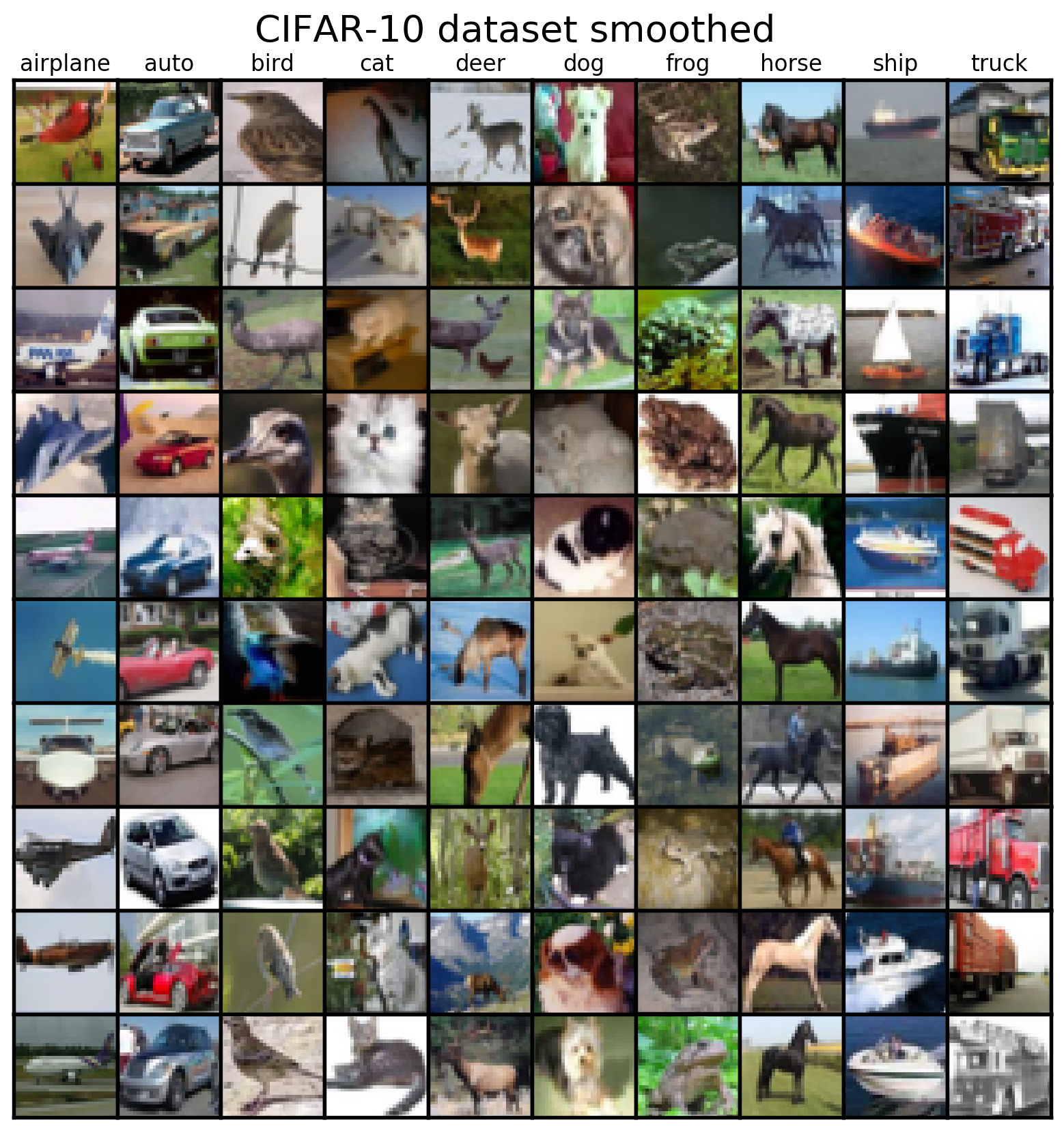
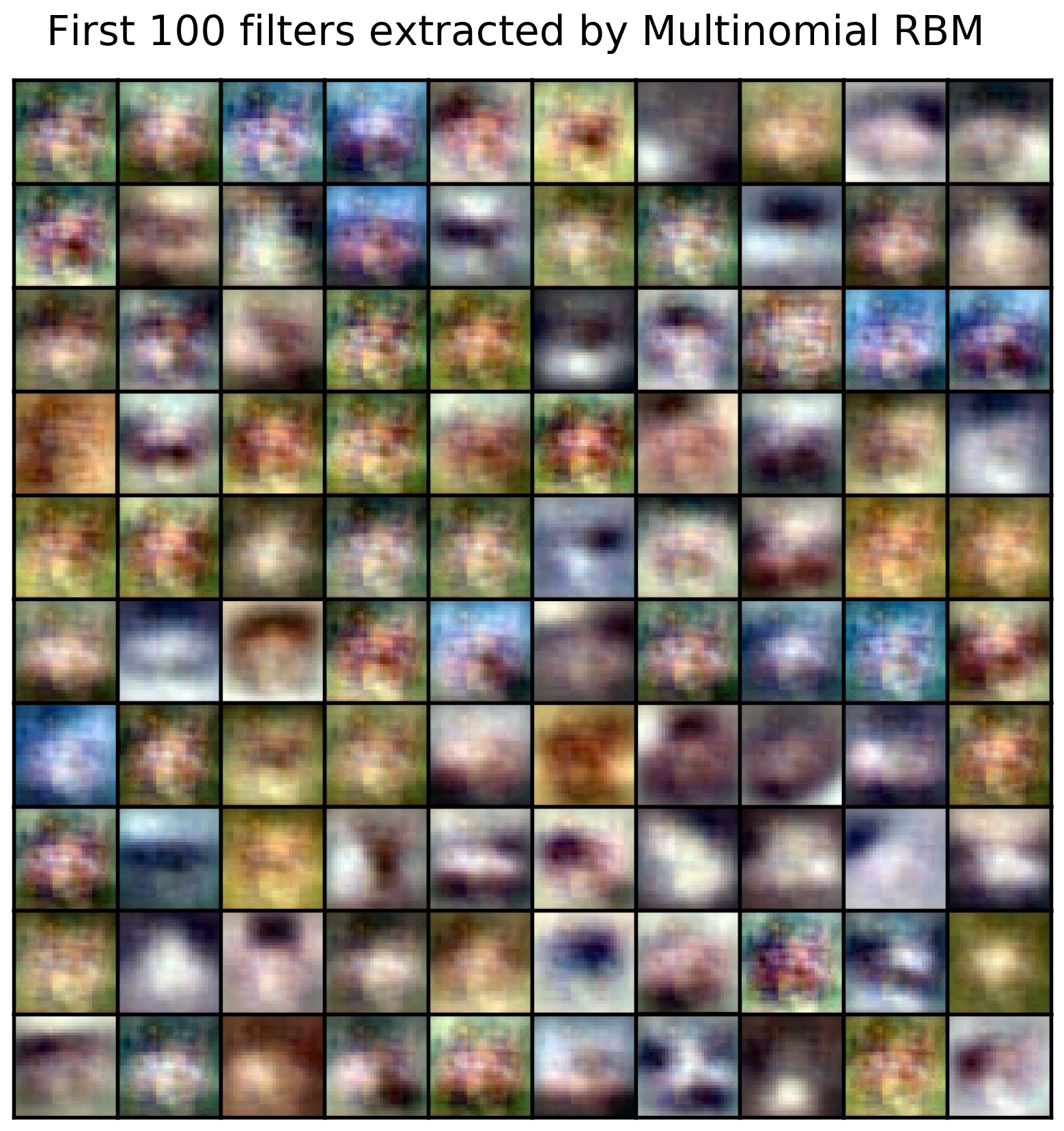
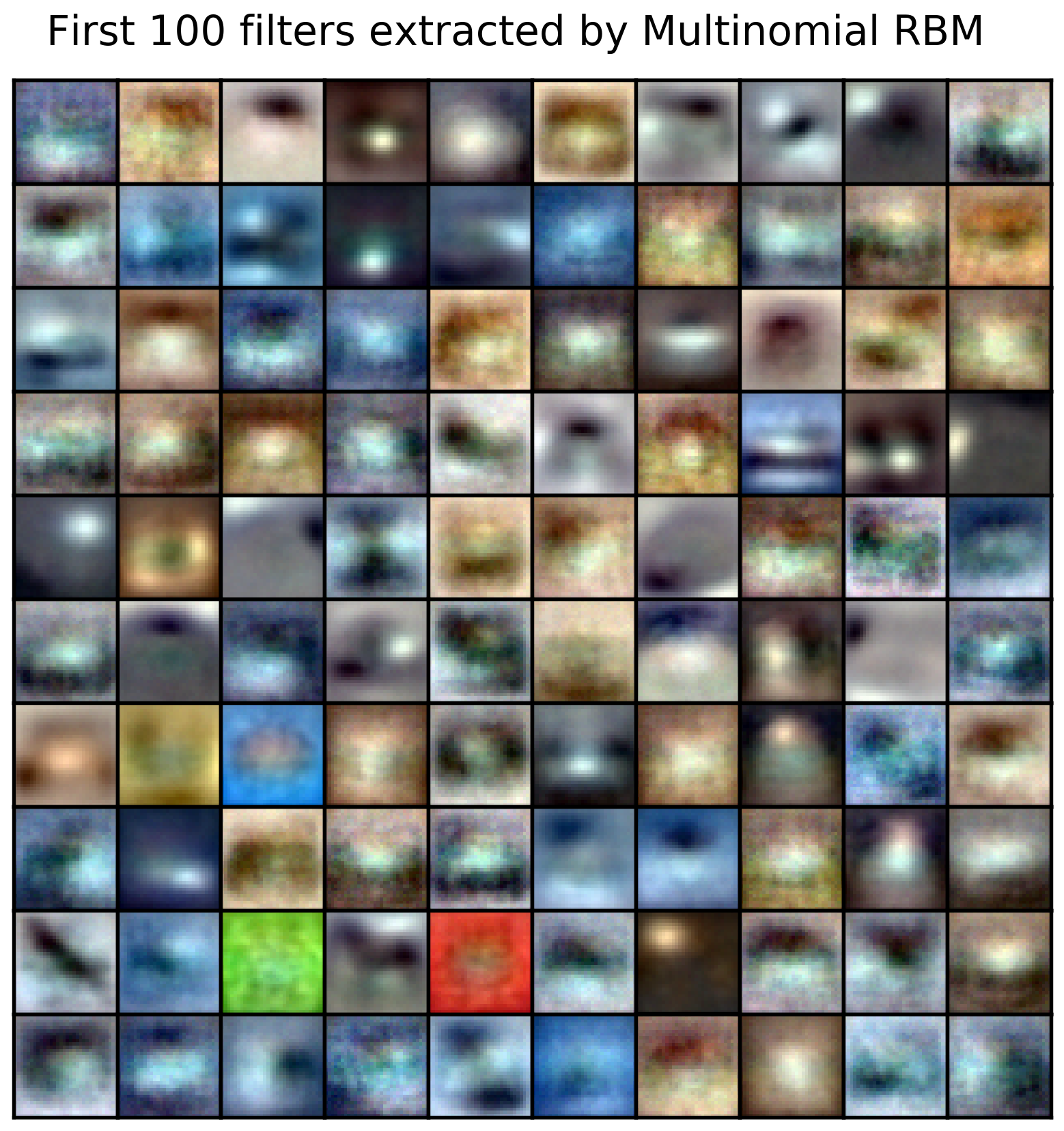
(Simply) train 3072-5000-1000 Gaussian-Bernoulli-Multinomial DBM on "smoothed" CIFAR-10 dataset (with 1000 least significant singular values removed, as suggested in [3]) with pre-training and:
- generate samples after training;
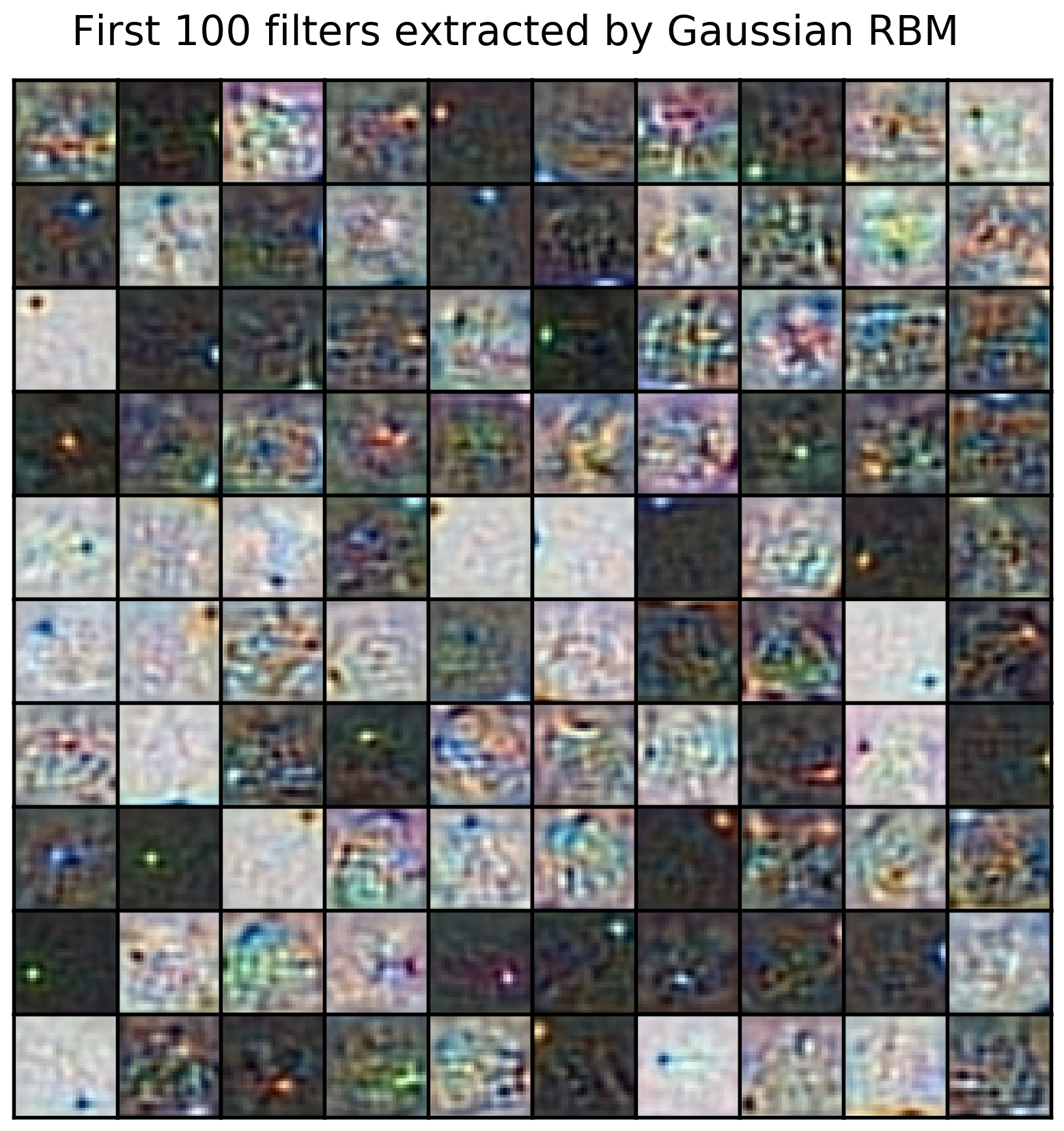
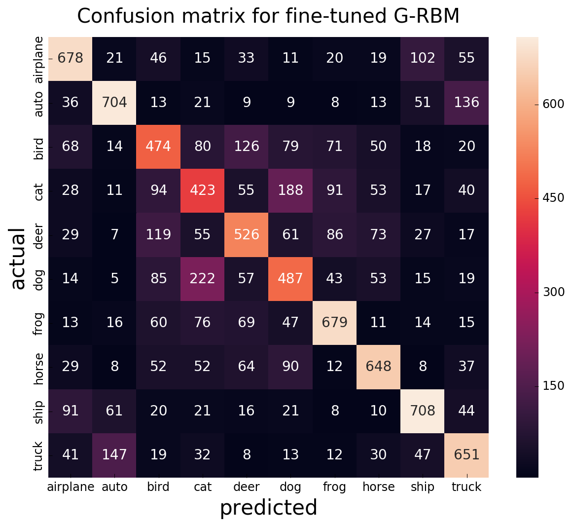
- use pre-trained Gaussian RBM (G-RBM) for classification.
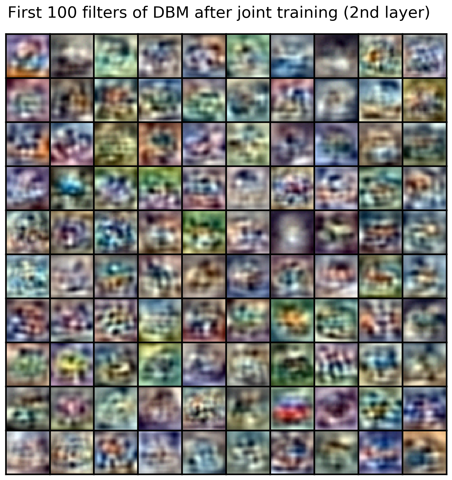
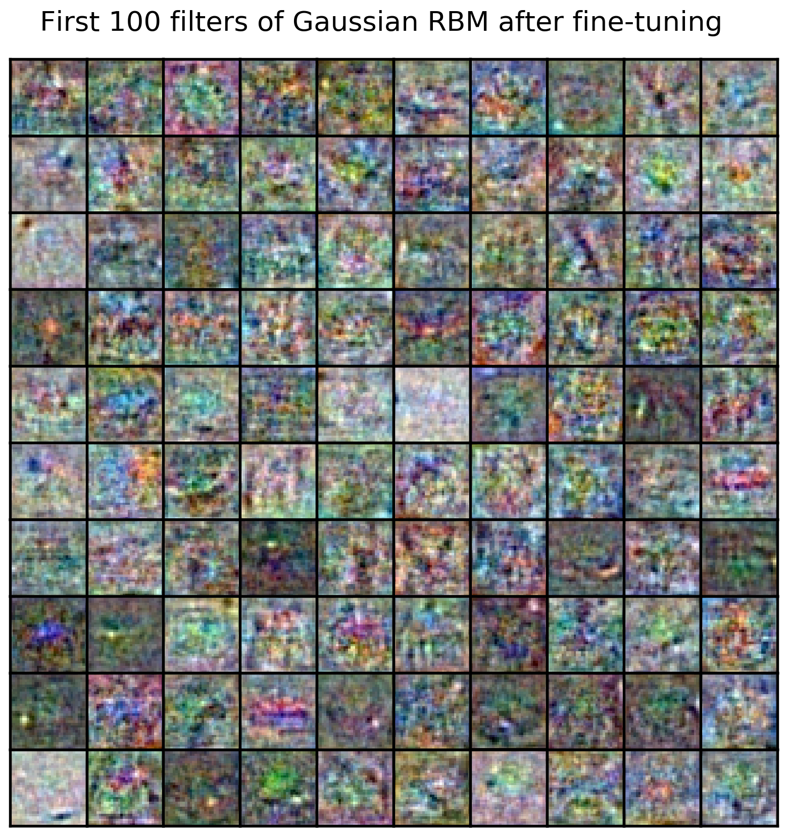
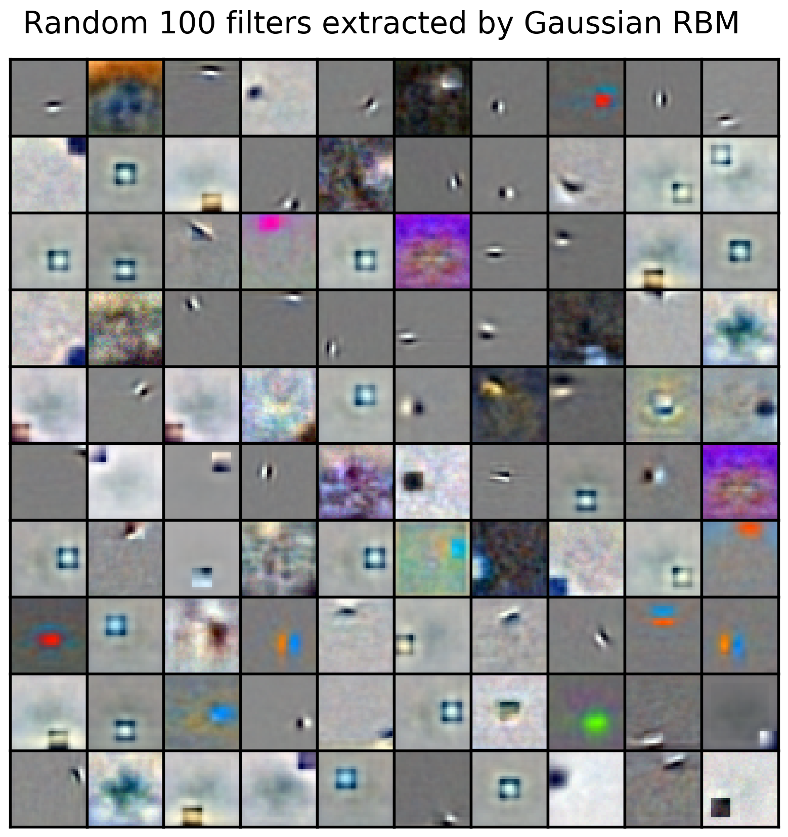
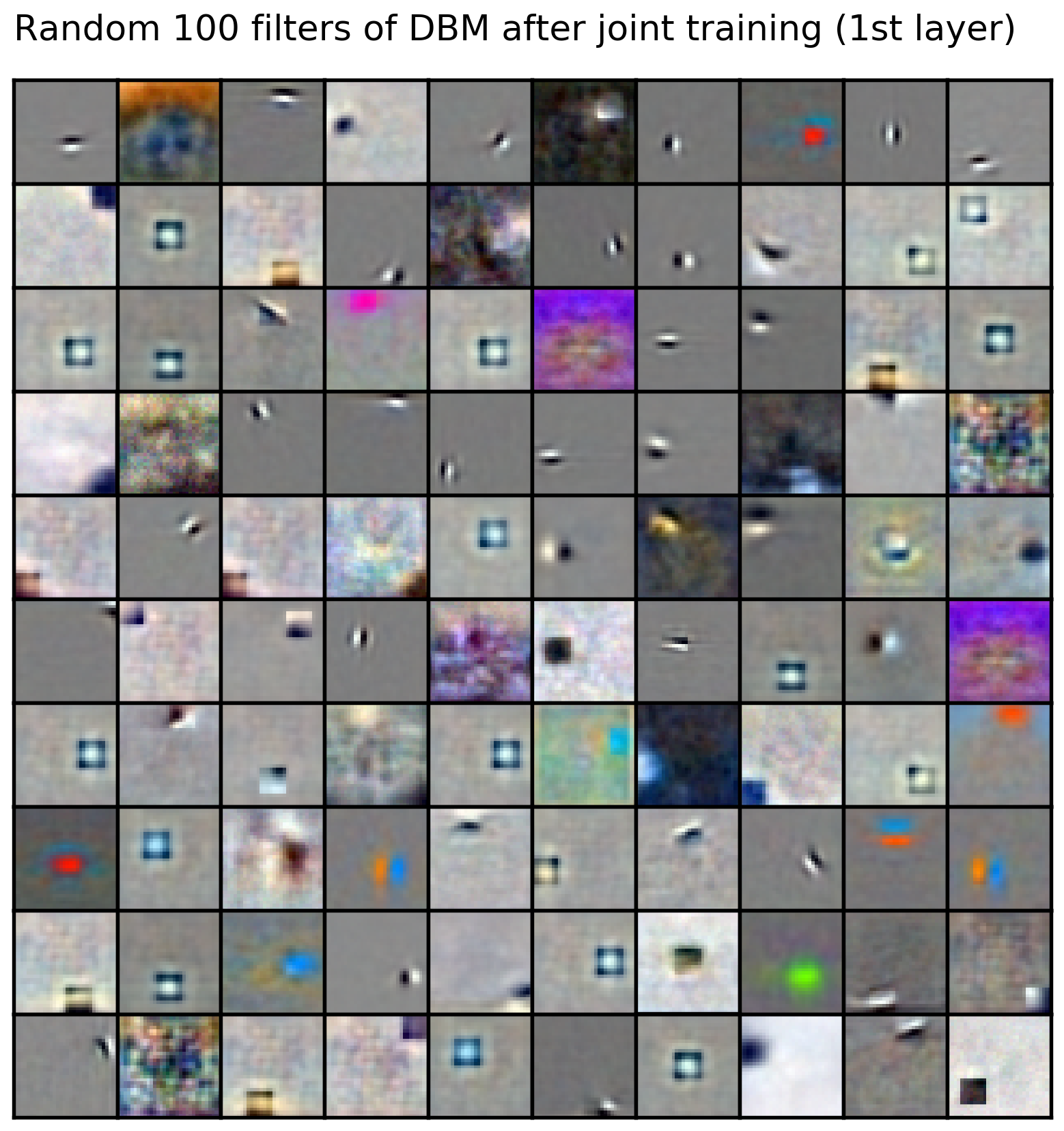
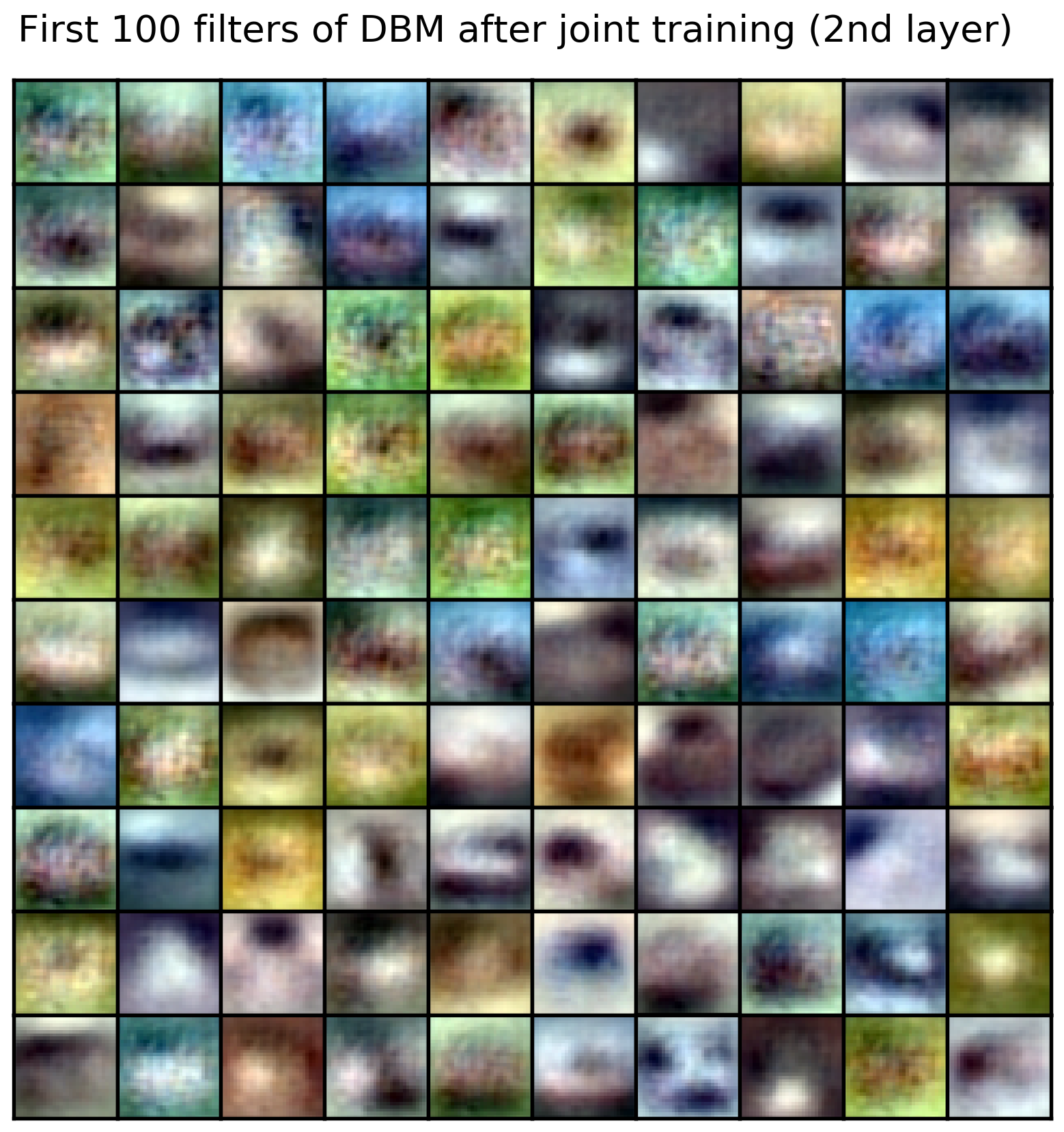
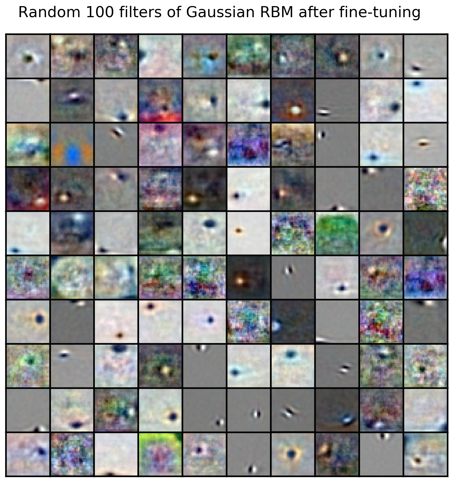
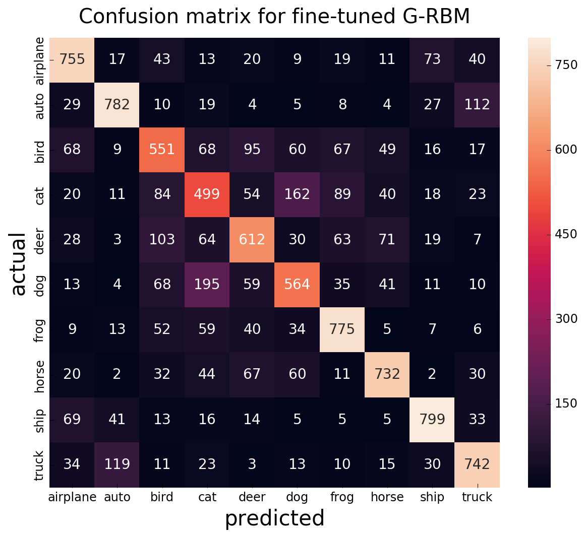
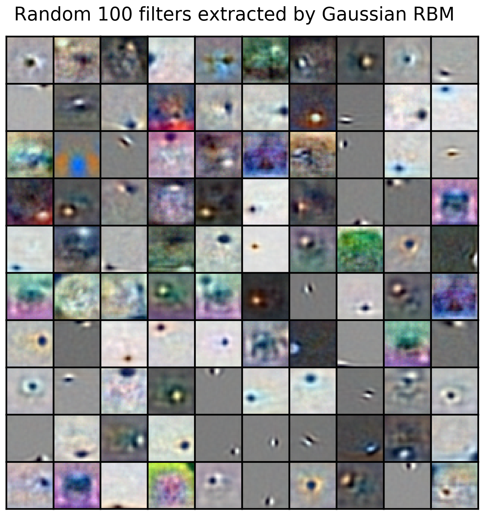
Despite poor-looking G-RBM features, classification performance after discriminative fine-tuning is much larger than reported backprop from random initialization [3], and is 5% behind best reported result using RBM (with twice larger number of hidden units). Note also that G-RBM is modified for DBM pre-training (notes or [1] for details):
algorithm |
test accuracy, % |
|---|---|
| Best known MLP w/o data augmentation: 8 layer ZLin net [6] | 69.62 |
| Best known method using RBM (w/o data augmentation?): 10k hiddens + fine-tuning [3] | 64.84 |
| Gaussian RBM + discriminative fine-tuning | 59.78 |
| Pure backprop 3072-5000-10 on smoothed data | 58.20 |
| Pure backprop 782-10k-10 on PCA whitened data [3] | 51.53 |
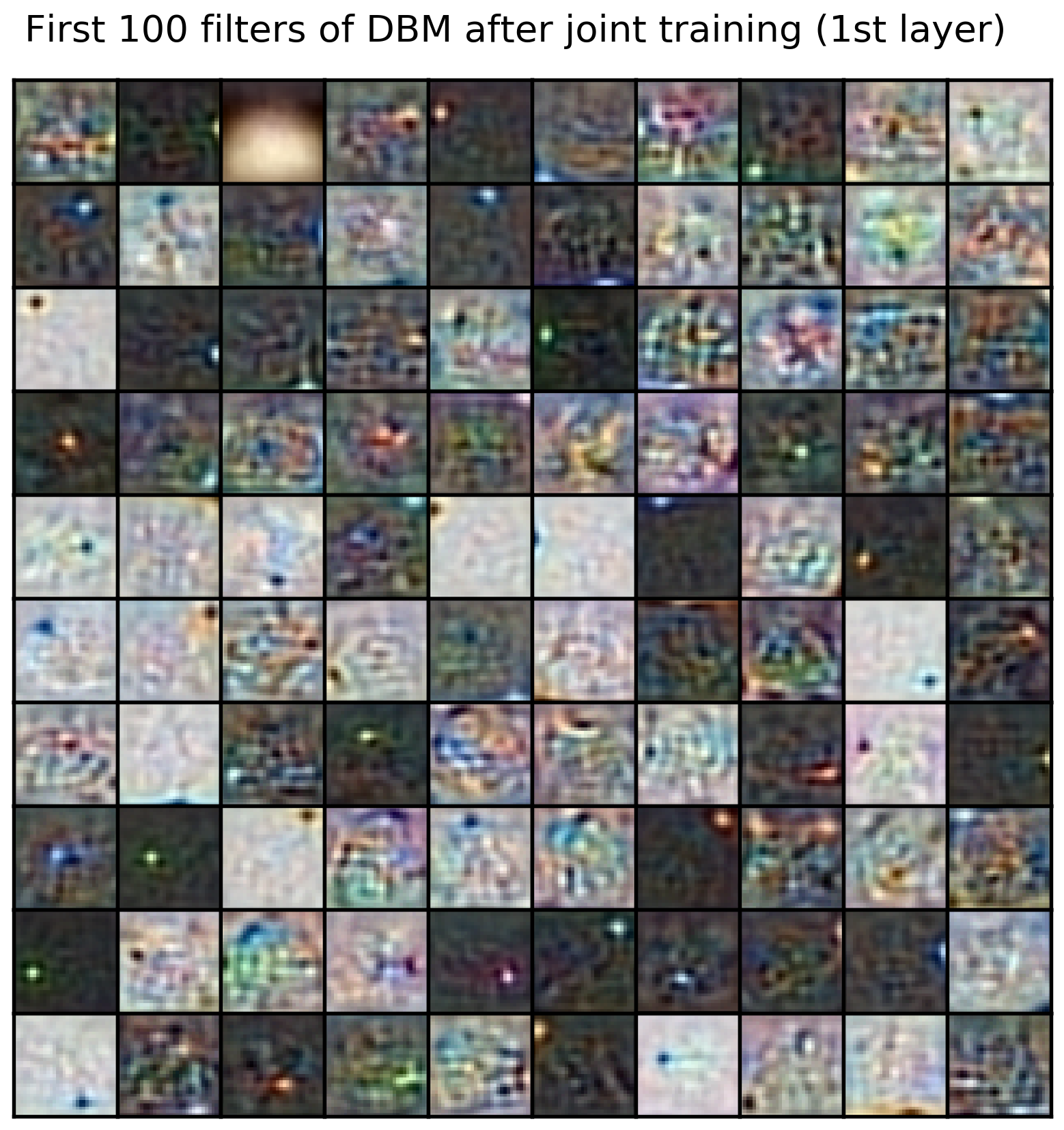
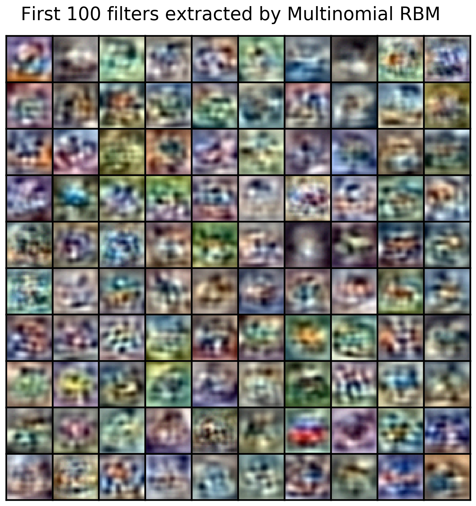
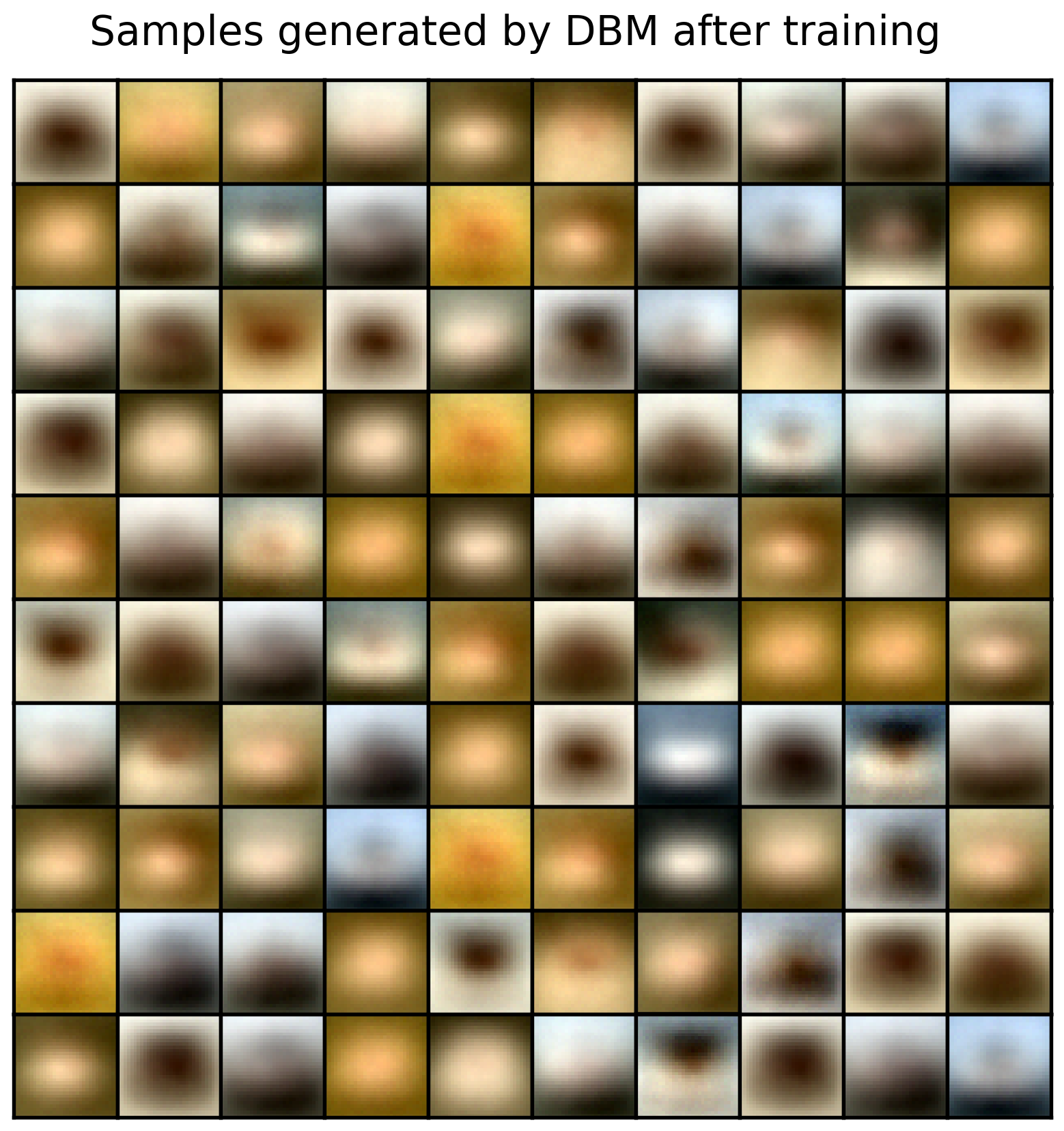
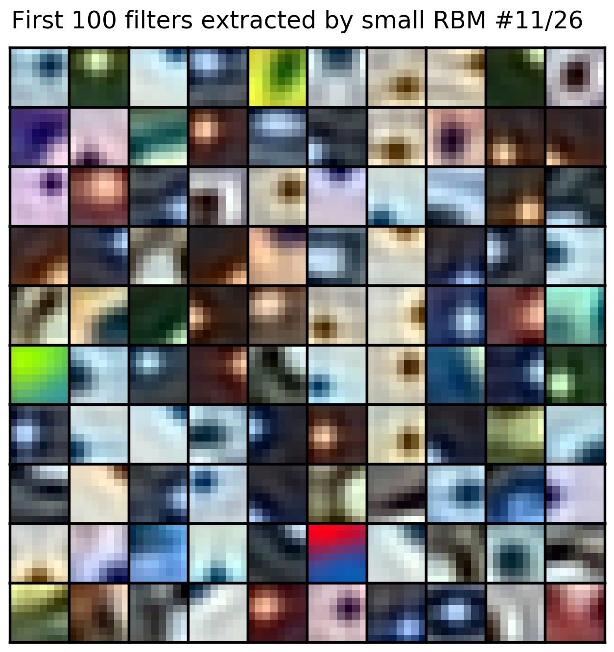
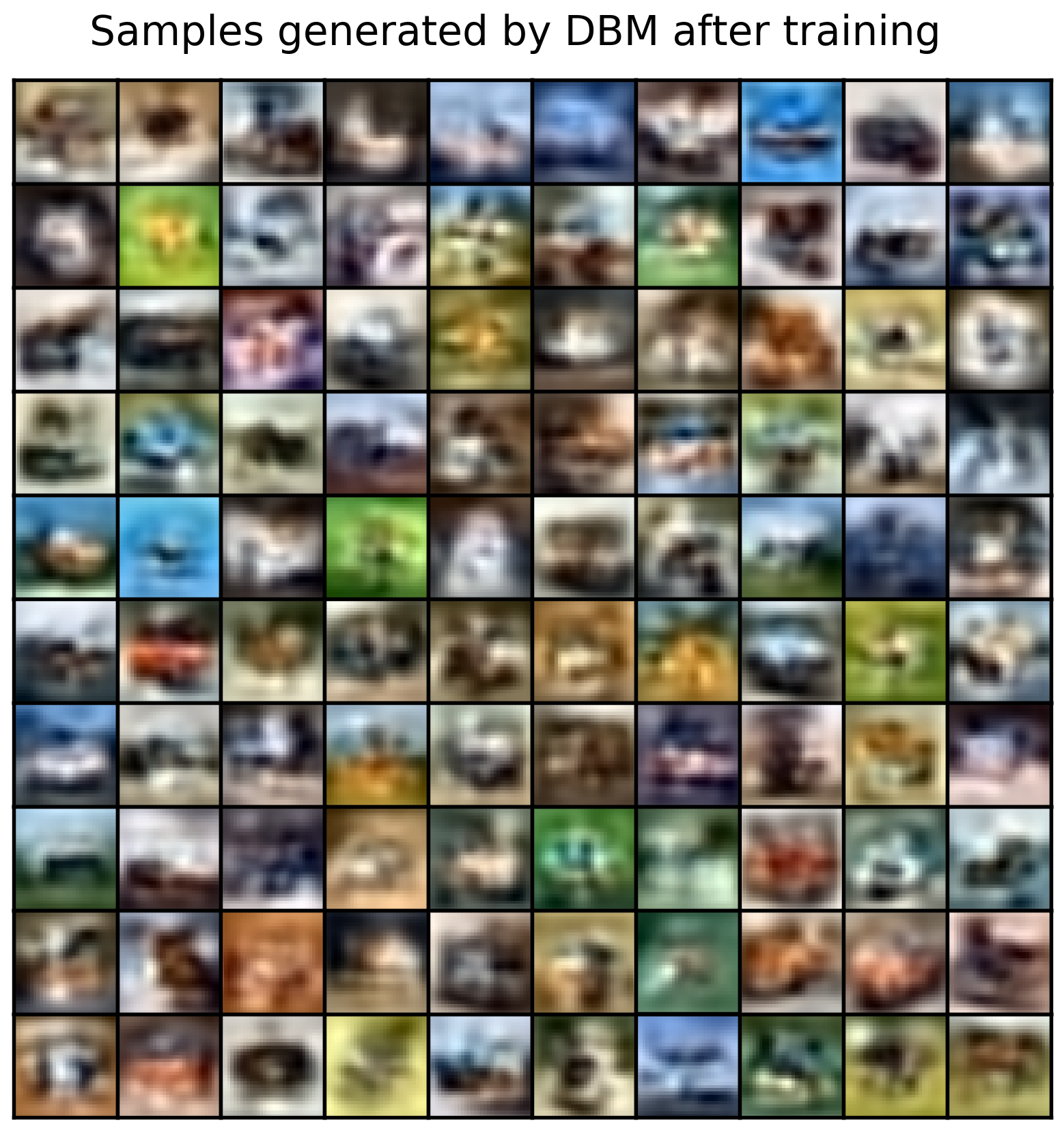
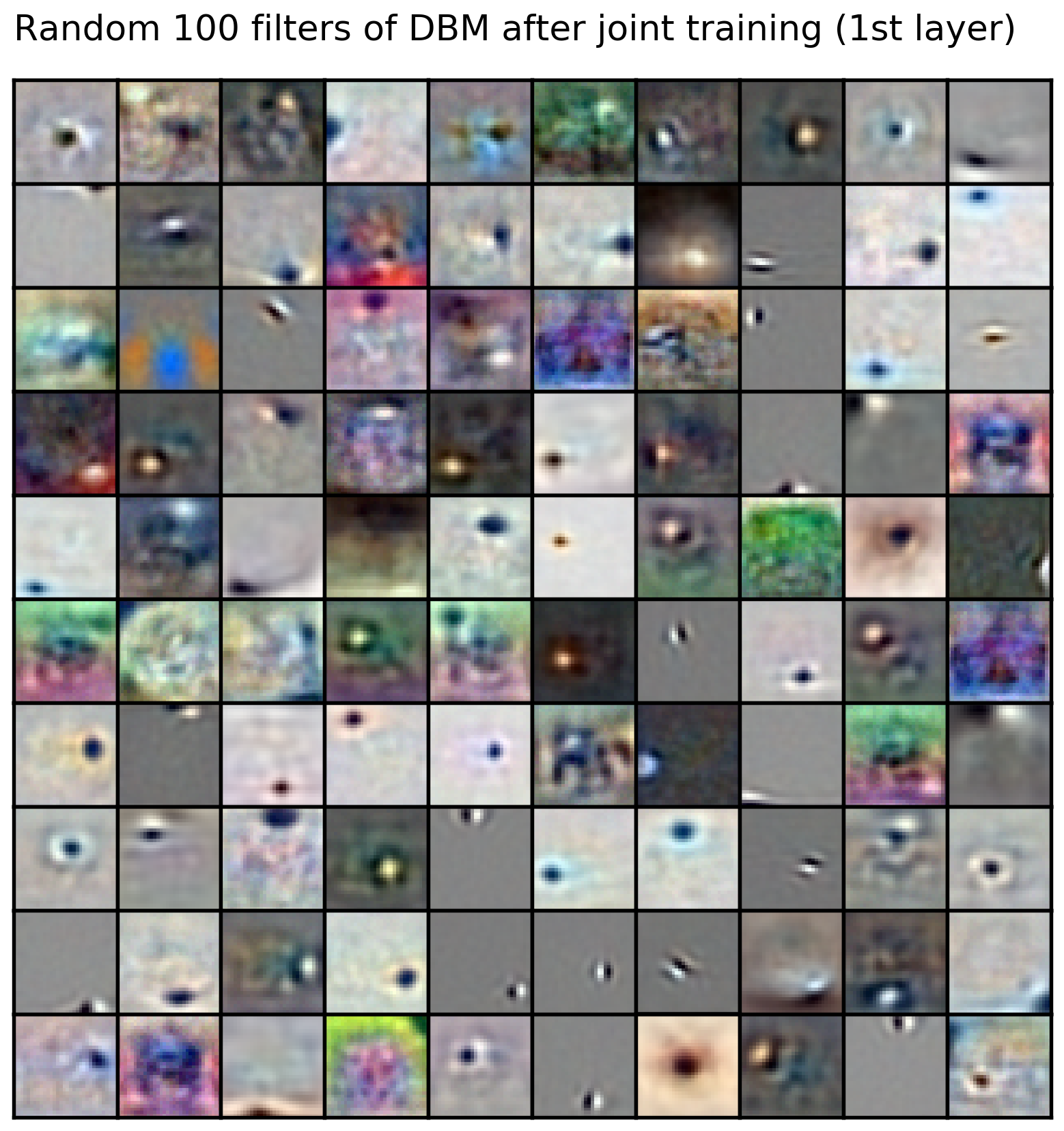
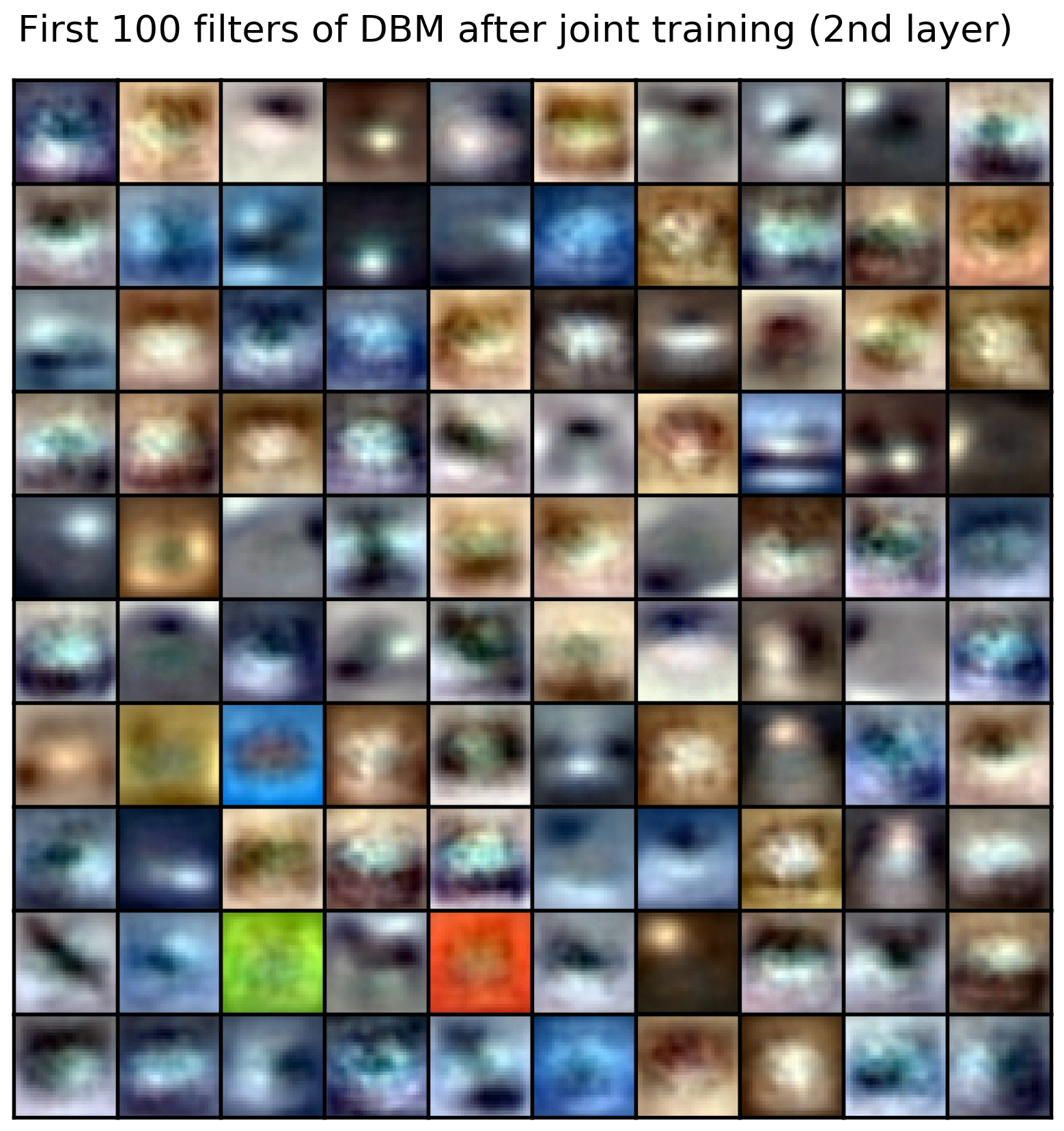
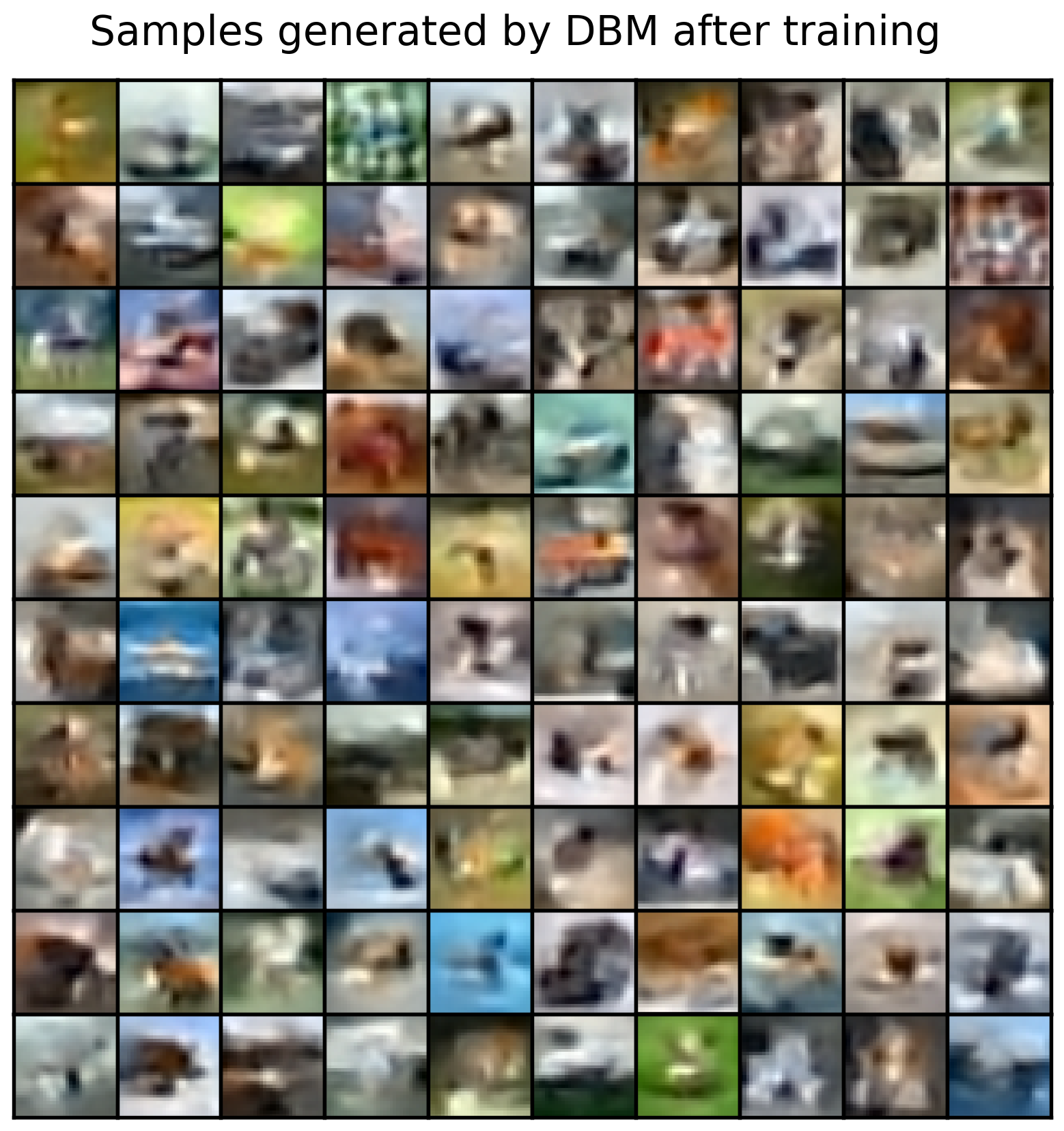
Train 3072-7800-512 G-B-M DBM with pre-training on CIFAR-10,
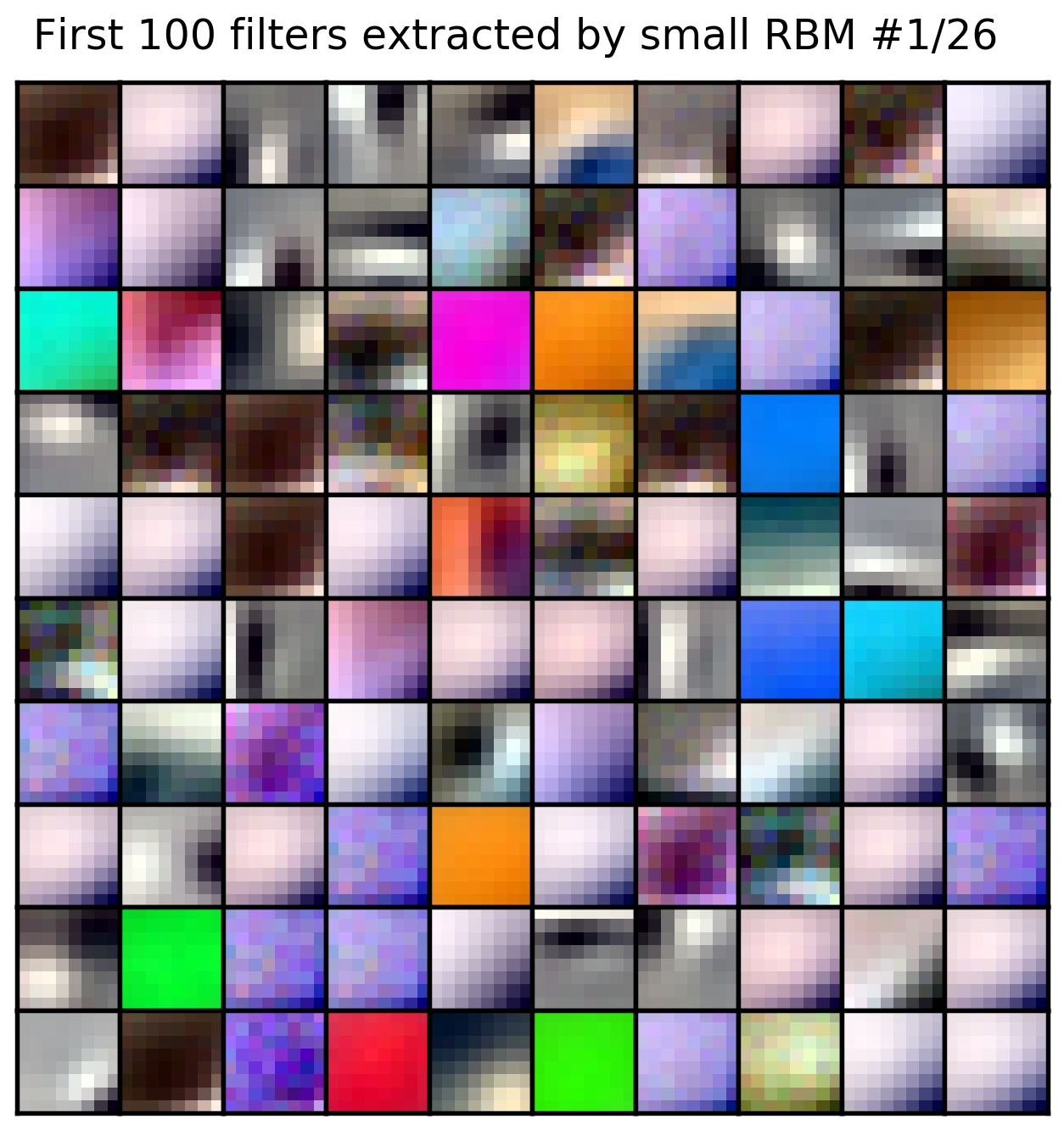
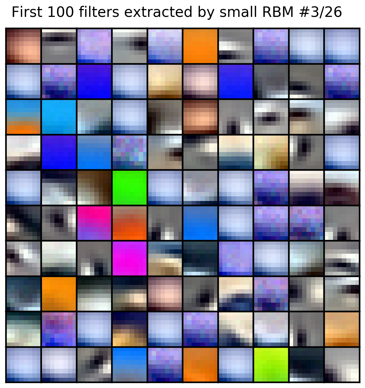
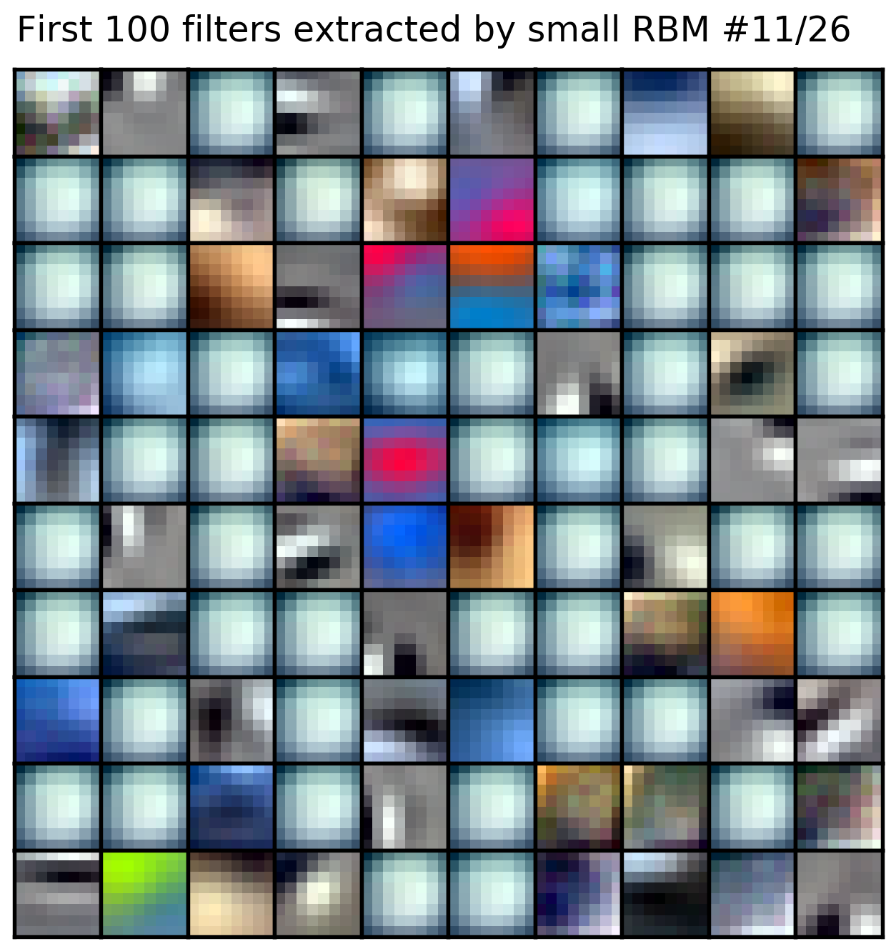
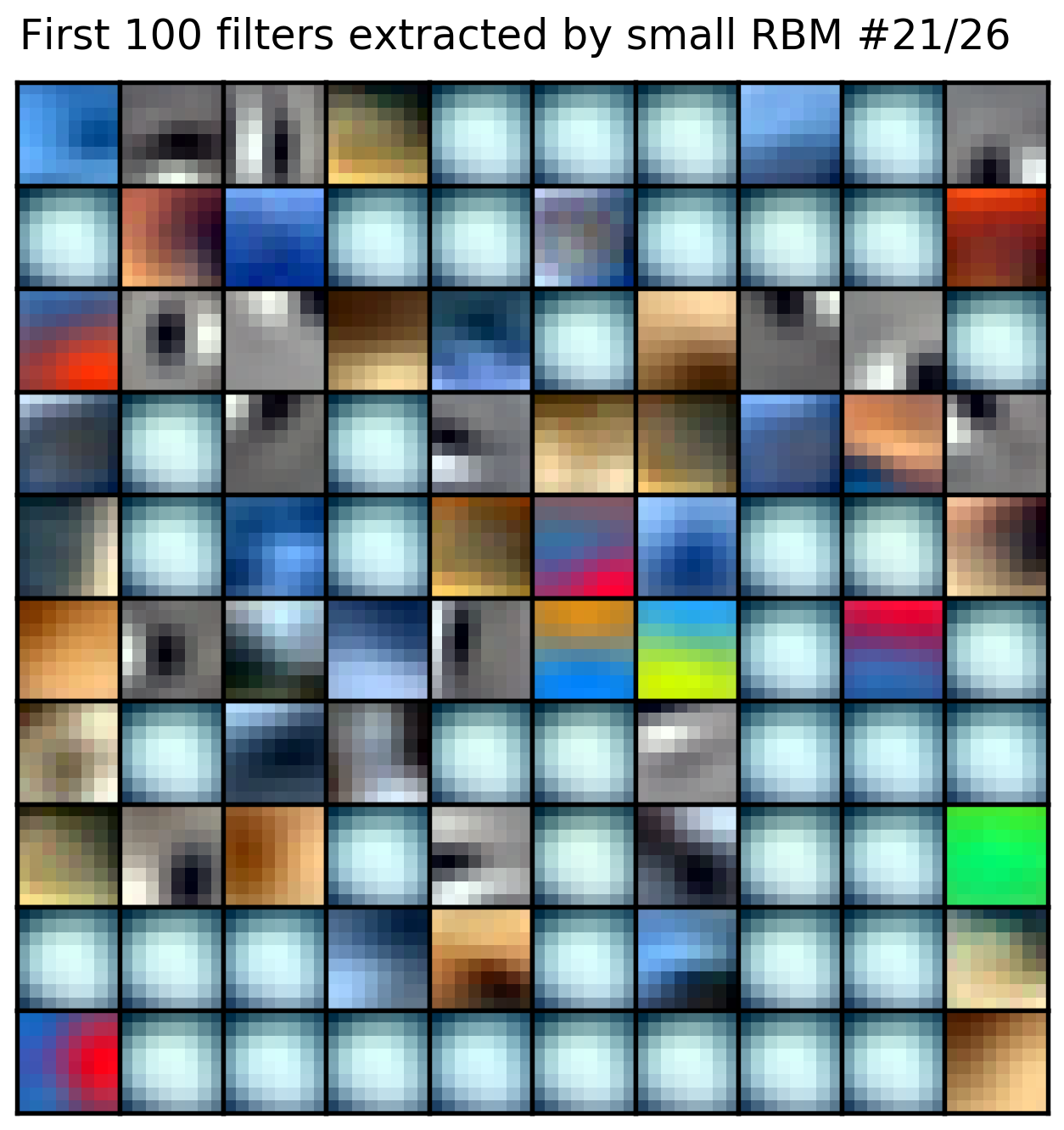
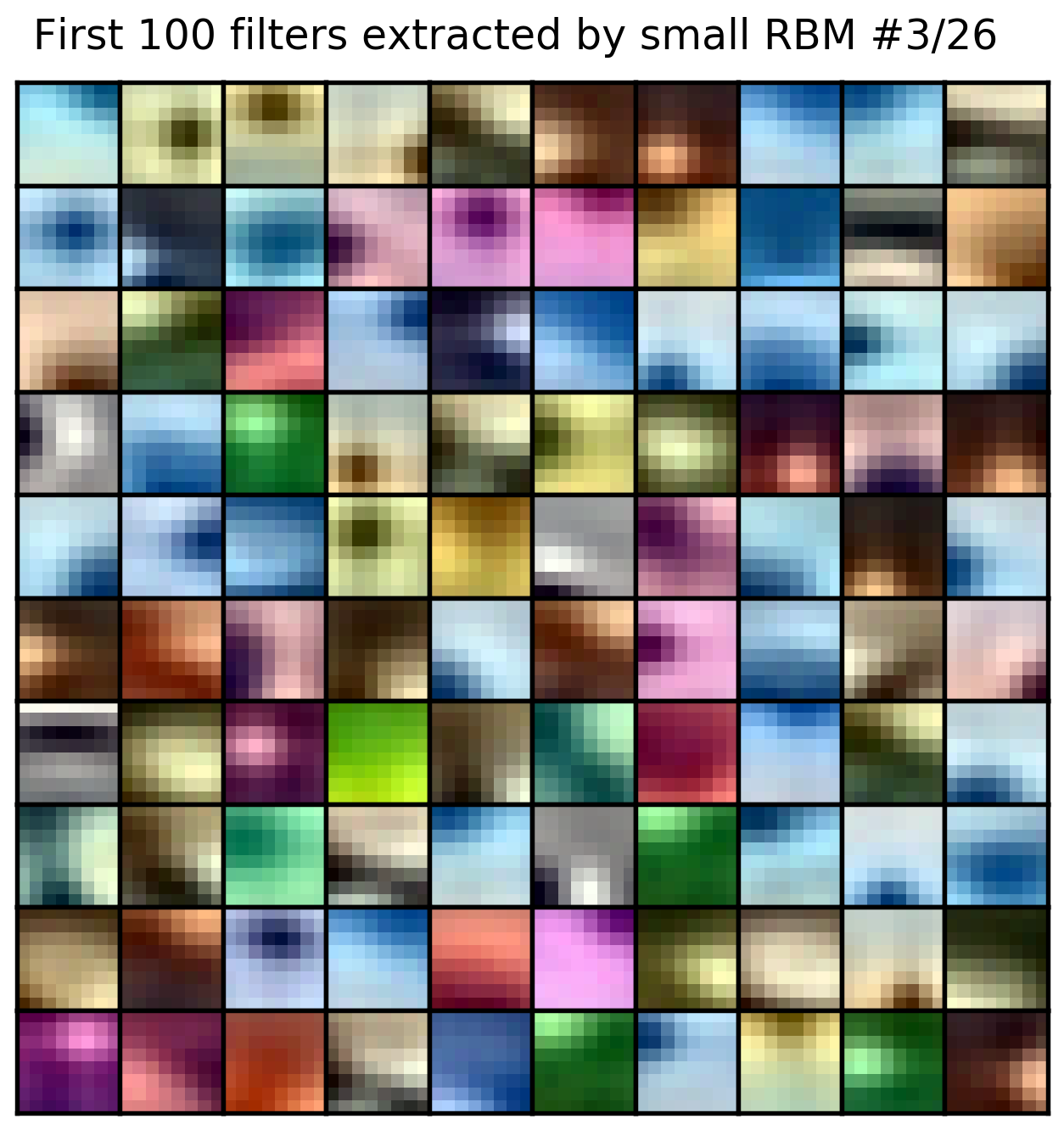
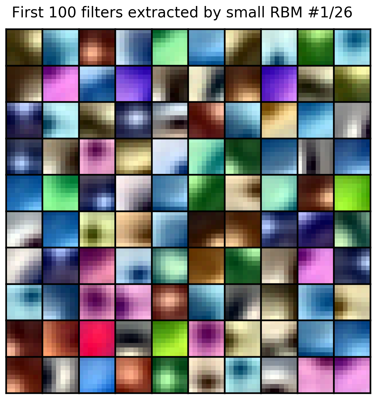
augmented (x10) using shifts by 1 pixel in all directions and horizontal mirroring and using more advanced training of G-RBM which is initialized from pre-trained 26 small RBM on patches of images, as in [3].
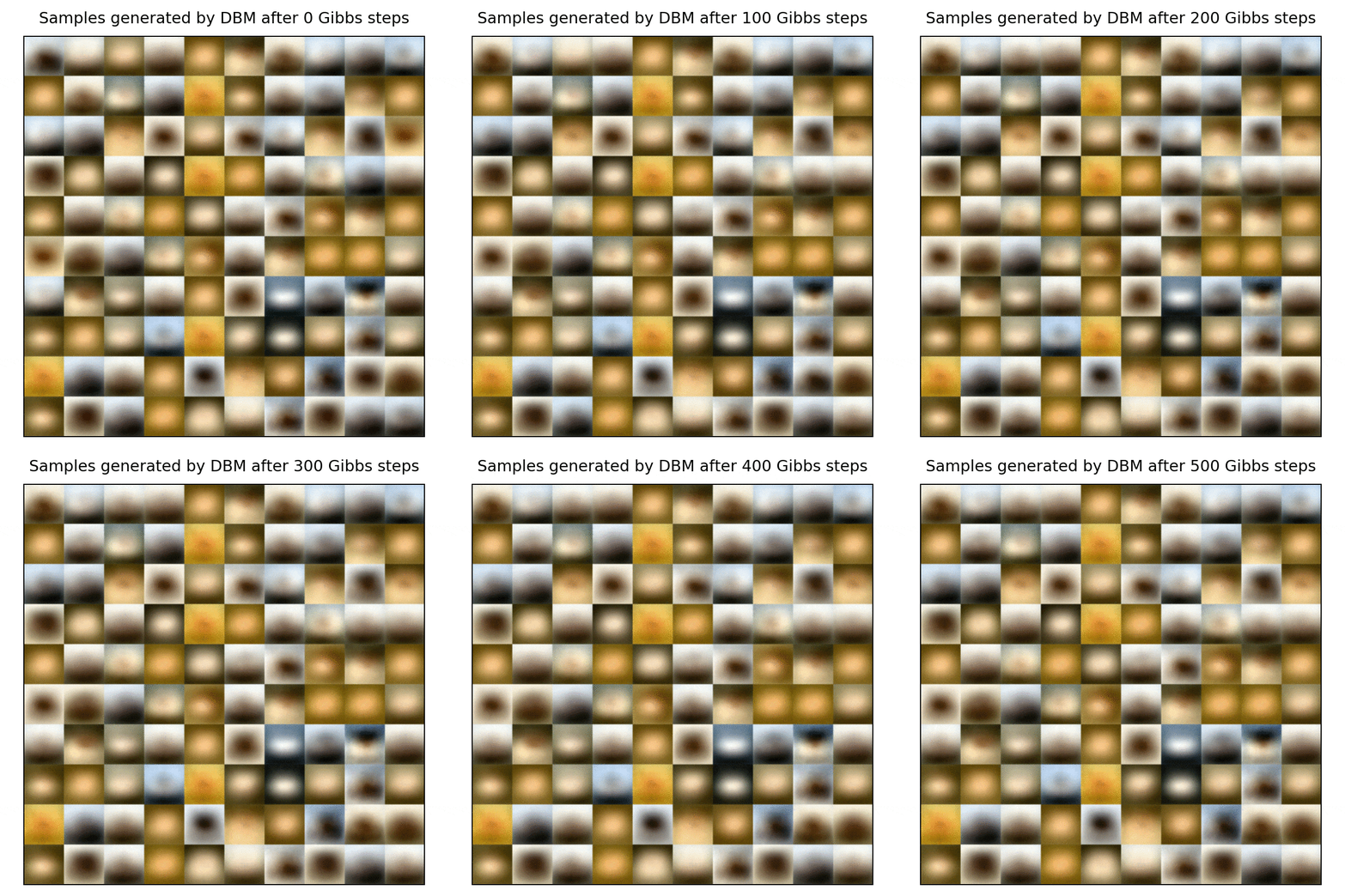
Notice how some of the particles are already resemble natural images of horses, cars etc. and note that the model is trained only on augmented CIFAR-10 (490k images), compared to 4M images that were used in [2].
I also trained for longer with
python dbm_cifar.py --small-l2 2e-3 --small-epochs 120 --small-sparsity-cost 0 \
                    --increase-n-gibbs-steps-every 20 --epochs 80 72 200 \
                    --l2 2e-3 0.01 1e-8 --max-mf-updates 70
While all RBMs have nicer features, this means that they overfit more than previously, and thus overall DBM performance is slightly worse.
The training with all pre-trainings takes quite a lot of time, but once trained, these nets can be used for other (similar) datasets/tasks.
Discriminative performance of Gaussian RBM now is very close to state of the art (having 7800 vs. 10k hidden units), and data augmentation given another 4% of test accuracy:
algorithm |
test accuracy, % |
|---|---|
| Gaussian RBM + discriminative fine-tuning + augmentation | 68.11 |
| Best known method using RBM (w/o data augmentation?): 10k hiddens + fine-tuning [3] | 64.84 |
| Gaussian RBM + discriminative fine-tuning | 64.38 |
| Gaussian RBM + discriminative fine-tuning (example #3) | 59.78 |
How to reproduce the this table see here.
Use scripts for training models from scratch, for instance
$ python rbm_mnist.py -h

(...)

usage: rbm_mnist.py [-h] [--gpu ID] [--n-train N] [--n-val N]
                    [--data-path PATH] [--n-hidden N] [--w-init STD]
                    [--vb-init] [--hb-init HB] [--n-gibbs-steps N [N ...]]
                    [--lr LR [LR ...]] [--epochs N] [--batch-size B] [--l2 L2]
                    [--sample-v-states] [--dropout P] [--sparsity-target T]
                    [--sparsity-cost C] [--sparsity-damping D]
                    [--random-seed N] [--dtype T] [--model-dirpath DIRPATH]
                    [--mlp-no-init] [--mlp-l2 L2] [--mlp-lrm LRM [LRM ...]]
                    [--mlp-epochs N] [--mlp-val-metric S] [--mlp-batch-size N]
                    [--mlp-save-prefix PREFIX]

optional arguments:
  -h, --help            show this help message and exit
  --gpu ID              ID of the GPU to train on (or '' to train on CPU)
                        (default: 0)
  --n-train N           number of training examples (default: 55000)
  --n-val N             number of validation examples (default: 5000)
  --data-path PATH      directory for storing augmented data etc. (default:
                        ../data/)
  --n-hidden N          number of hidden units (default: 1024)
  --w-init STD          initialize weights from zero-centered Gaussian with
                        this standard deviation (default: 0.01)
  --vb-init             initialize visible biases as logit of mean values of
                        features, otherwise (if enabled) zero init (default:
                        True)
  --hb-init HB          initial hidden bias (default: 0.0)
  --n-gibbs-steps N [N ...]
                        number of Gibbs updates per weights update or sequence
                        of such (per epoch) (default: 1)
  --lr LR [LR ...]      learning rate or sequence of such (per epoch)
                        (default: 0.05)
  --epochs N            number of epochs to train (default: 120)
  --batch-size B        input batch size for training (default: 10)
  --l2 L2               L2 weight decay coefficient (default: 1e-05)
  --sample-v-states     sample visible states, otherwise use probabilities w/o
                        sampling (default: False)
  --dropout P           probability of visible units being on (default: None)
  --sparsity-target T   desired probability of hidden activation (default:
                        0.1)
  --sparsity-cost C     controls the amount of sparsity penalty (default:
                        1e-05)
  --sparsity-damping D  decay rate for hidden activations probs (default: 0.9)
  --random-seed N       random seed for model training (default: 1337)
  --dtype T             datatype precision to use (default: float32)
  --model-dirpath DIRPATH
                        directory path to save the model (default:
                        ../models/rbm_mnist/)
  --mlp-no-init         if enabled, use random initialization (default: False)
  --mlp-l2 L2           L2 weight decay coefficient (default: 1e-05)
  --mlp-lrm LRM [LRM ...]
                        learning rate multipliers of 1e-3 (default: (0.1,
                        1.0))
  --mlp-epochs N        number of epochs to train (default: 100)
  --mlp-val-metric S    metric on validation set to perform early stopping,
                        {'val_acc', 'val_loss'} (default: val_acc)
  --mlp-batch-size N    input batch size for training (default: 128)
  --mlp-save-prefix PREFIX
                        prefix to save MLP predictions and targets (default:
                        ../data/rbm_)
or download pretrained ones with default parameters using models/fetch_models.sh,
and check notebooks for corresponding inference / visualizations etc.
Note that training is skipped if there is already a model in model-dirpath, and similarly for other experiments (you can choose different location for training another model).
- GPU memory: at most 2-3 GB for each model in each example, and it is always possible to decrease batch size and number of negative particles;
- RAM: at most 11GB (to run last example, features from Gaussian RBM are in
halfprecision) and (much) lesser for other examples.
All models from all experiments can be downloaded by running models/fetch_models.sh or manually from Google Drive.
Also, you can download additional data (fine-tuned models' predictions, fine-tuned weights, means and standard deviations for datasets for examples #3, #4) using data/fetch_additional_data.sh
Check also my supplementary notes (or dropbox) with some historical outlines, theory, derivations, observations etc.
By default, the following commands install (among others) tensorflow-gpu~=1.3.0. If you want to install tensorflow without GPU support, replace corresponding line in requirements.txt. If you have already tensorflow installed, comment that line.
git clone https://github.com/monsta-hd/boltzmann-machines.git
cd boltzmann-machines
pip install -r requirements.txt
See here how to run from a virtual environment.
See here how to run from a docker container.
To run some notebooks you also need to install JSAnimation:
git clone https://github.com/jakevdp/JSAnimation
cd JSAnimation
python setup.py install
After installation, tests can be run with:
make testAll the necessary data can be downloaded with:
make dataImportError: libcudnn.so.6: cannot open shared object file: No such file or directory.
TensorFlow 1.3.0 assumes cuDNN v6.0 by default. If you have different one installed, you can create symlink to libcudnn.so.6 in /usr/local/cuda/lib64 or /usr/local/cuda-8.0/lib64. More details here.
- add stratification;
- add t-SNE visualization for extracted features;
- generate half MNIST digit conditioned on the other half using RBM;
- implement Centering [7] for all models;
- implement classification RBMs/DBMs?;
- implement ELBO and AIS for arbitrary DBM (again, visible and topmost hidden units can be analytically summed out);
- optimize input pipeline e.g. use queues instead of
feed_dictetc.
Feel free to improve existing code, documentation or implement new feature (including those listed in Possible future work). Please open an issue to propose your changes if they are big enough.
[1] R. Salakhutdinov and G. Hinton. Deep boltzmann machines. In: Artificial Intelligence and Statistics, pages 448–455, 2009. [PDF]
[2] R. Salakhutdinov, J. B. Tenenbaum, and A. Torralba. Learning with hierarchical-deep models. IEEE transactions on pattern analysis and machine intelligence, 35(8):1958–1971, 2013. [PDF]
[3] A. Krizhevsky and G. Hinton. Learning multiple layers of features from tiny images. 2009. [PDF]
[4] G. Hinton. A practical guide to training restricted boltzmann machines. Momentum, 9(1):926, 2010. [PDF]
[5] R. Salakhutdinov and I. Murray. On the quantitative analysis of Deep Belief Networks. In A. McCallum and S. Roweis, editors, Proceedings of the 25th Annual International Conference on Machine Learning (ICML 2008), pages 872–879. Omnipress, 2008 [PDF]
[6] Lin Z, Memisevic R, Konda K. How far can we go without convolution: Improving fully-connected networks, ICML 2016. [arXiv]
[7] G. Montavon and K.-R. Müller. Deep boltzmann machines and the centering trick. In Neural Networks: Tricks of the Trade, pages 621–637. Springer, 2012. [PDF]
![Free energy gap [4]](https://raw.githubusercontent.com/enijkamp/rbm/master/img/tensorboard_rbm/feg.png)
