DOTA or more specifically DOTA 2 is an online MOBA (Massive online battle arena) game developed and hosted by Valve Corporation. Dota 2 has a widespread and active competitive scene, with teams from across the world playing professionally in various dedicated leagues and tournaments. Premium Dota 2 tournaments often have prize pools totaling millions of US dollars, the highest of any eSport.
In DOTA there are two opposing teams called Radiant and Dire trying to destroy the opposing team's base. During the game the players collecting experience points to level up and gain additional skills and also gold to buy equipment. Additional details can be found here: Wikipedia, DOTA 2 Wiki
The goal of this experiment is to find a model that could estimate the outcome of a DOTA 2 match based only on the participating players and their stats/history and on the information that is available only at the beginning of the matches.
Data was downloaded from https://www.kaggle.com/devinanzelmo/dota-2-matches The downloaded data has to be extracted to a data folder in the working directory.
The data consists multiple files but only some of them were used. Please find detailed description below.
library(readr)
library(data.table)
library(reshape2)
library(dplyr)
library(h2o)
library(ggplot2)
library(gridExtra)

localH2O = h2o.init(nthreads=-1)

##  Connection successful!
##
## R is connected to the H2O cluster:
##     H2O cluster uptime:         2 hours 31 minutes
##     H2O cluster version:        3.10.3.4
##     H2O cluster version age:    1 month and 16 days
##     H2O cluster name:           H2O_started_from_R_Janos_Strasszer_cvj821
##     H2O cluster total nodes:    1
##     H2O cluster total memory:   3.15 GB
##     H2O cluster total cores:    4
##     H2O cluster allowed cores:  4
##     H2O cluster healthy:        TRUE
##     H2O Connection ip:          localhost
##     H2O Connection port:        54321
##     H2O Connection proxy:       NA
##     R Version:                  R version 3.3.2 (2016-10-31)
Match contains all the high level statistics of the match like the status of the towers at the end of the match and more importantly the outcome. Most if these variables should be dropped because most of them are not available before the matches.
The few exceptions:
game_mode:
match <- data.table(read_csv("data/match.csv"))
nrow(match)

## [1] 50000

match[, .N, by=game_mode]

##    game_mode     N
## 1:        22 48670
## 2:         2  1330
The two possible values for game_mode are the same from the aspect of game mechanics. Both (2-Captain Mode, 22-Ranked Matchmaking) are consists of a banning phase followed by all pick --> Feature will be removed.
start_time: It is irrelevant --> Will be removed.
radiant_win: Indicates whether the Radiant or the Dire team won the match. It will be converted to a binary variable: 1-Radiant, 0-Dire win.
match_id: should be kept to identify the match.
Finalize match outcome df:
# Training outcome
match <- match[, list(match_id,radiant_win)]
match[, winner:= as.factor(if_else(radiant_win == "True", true = "RADIANT", false = "DIRE"))]

##        match_id radiant_win  winner
##     1:        0        True RADIANT
##     2:        1       False    DIRE
##     3:        2       False    DIRE
##     4:        3       False    DIRE
##     5:        4        True RADIANT
##    ---
## 49996:    49995        True RADIANT
## 49997:    49996        True RADIANT
## 49998:    49997        True RADIANT
## 49999:    49998        True RADIANT
## 50000:    49999       False    DIRE

match$radiant_win <- NULL
ranked_match_outcome_train <- match
rm(match)

# Test outcome
ranked_match_outcome_test <- data.table(read_csv("data/test_labels.csv"))
ranked_match_outcome_test[, winner:=as.factor(if_else(radiant_win == 1, true = "RADIANT", false = "DIRE"))]

##         match_id radiant_win  winner
##      1:    50000           0    DIRE
##      2:    50001           1 RADIANT
##      3:    50002           0    DIRE
##      4:    50003           1 RADIANT
##      5:    50004           0    DIRE
##     ---
##  99996:   149995           1 RADIANT
##  99997:   149996           1 RADIANT
##  99998:   149997           1 RADIANT
##  99999:   149998           1 RADIANT
## 100000:   149999           0    DIRE

ranked_match_outcome_test$radiant_win <- NULL
test_labels.csv has a similar structure but only contains the outcome of the matches. It is ideal to be used as validation data.
legacy_player_ratings <- data.table(read_csv("data/player_ratings.csv"))
nrow(legacy_player_ratings)

## [1] 834226
total_wins: The total number of wins the player has.
total_matches: The total number of matches the player played.
Contains player information for the matches: What player played what hero in what slot. Also there are a tons of performance indicators that won't be listed here but later during the experiments. For more information please check the data description on Kaggle.
test_player.csv has similar information but without the performance indicators thus it is ideal to be used as validation data.
In the first experiment only the average player winrate per team will be used as feature in the prediction.
# Player ratings can be calculated from 900K historical matches
legacy_player_ratings[, win_percent:=total_wins/total_matches]

##         account_id total_wins total_matches trueskill_mu trueskill_sigma
##      1:     236579         14            24     27.86804        5.212361
##      2:       -343          1             1     26.54416        8.065475
##      3:      -1217          1             1     26.52110        8.114989
##      4:      -1227          1             1     27.24802        8.092217
##      5:      -1284          0             1     22.93102        8.092224
##     ---
## 834222: -298722891          1             1     27.64315        8.013786
## 834223:     106173          0             1     23.06938        7.998792
## 834224:     312076          1             1     28.21708        7.889176
## 834225: -299193988          0             2     22.40614        7.851303
## 834226:          0    1608398       3315071     25.00000        8.333333
##         win_percent
##      1:   0.5833333
##      2:   1.0000000
##      3:   1.0000000
##      4:   1.0000000
##      5:   0.0000000
##     ---
## 834222:   1.0000000
## 834223:   0.0000000
## 834224:   1.0000000
## 834225:   0.0000000
## 834226:   0.4851775

# Imputing missing data: if there is no stat for the player, lets asume he is an average player (id 0 is for the average)
unidentified_win_percent <- legacy_player_ratings[account_id==0, win_percent]

# Each row represents a player in a match thus 10 rows represents a match
players_train <- data.table(read_csv("data/players.csv"))
players_test <- data.table(read_csv("data/test_player.csv"))

feature1 <- function(legacy_player_ratings, players, outcome, imputed_win_percent) {
  playerdata <- data.table(left_join(players, legacy_player_ratings[, c("account_id", "win_percent")],
                          by=c("account_id" = "account_id")))
  playerdata[is.na(win_percent), win_percent:=unidentified_win_percent]

  # player_slot 0-4: radiant, 128-132: dire
  playerdata[, side:= as.factor(if_else(player_slot < 100, true = "RADIANT", false = "DIRE"))]

  teamstat <- playerdata%>% group_by(match_id, side) %>% summarise(win_percent_legacy=mean(win_percent))
  teamstat <- left_join(teamstat[teamstat$side == "RADIANT", c("match_id", "win_percent_legacy")],
                  teamstat[teamstat$side == "DIRE", c("match_id", "win_percent_legacy")],
                  by="match_id", suffix=c("_RADIANT", "_DIRE"))
  out <- left_join(outcome, teamstat, by="match_id")

  return(out)
}

train <- feature1(legacy_player_ratings, players_train, ranked_match_outcome_train, unidentified_win_percent)
test <- feature1(legacy_player_ratings, players_test, ranked_match_outcome_test, unidentified_win_percent)
Try to do the analysis
upload_data <- function(up_train, up_test) {
  if(exists("h_train")) {
    h2o.rm(h_train)
  }
  if(exists("h_test")) {
    h2o.rm(h_test)
  }
  h_train <<- as.h2o(up_train)
  h_test <<- as.h2o(up_test)
}

upload_data(train, test)

linear_model <- h2o.glm(x = c("win_percent_legacy_RADIANT", "win_percent_legacy_DIRE"), y = "winner",
                  training_frame = h_train, validation_frame = h_test,
                  family = "binomial",
                  score_each_iteration = TRUE)

model_performance <- function(model) {
  auc <- h2o.auc(model, valid = TRUE)
  fpr <- h2o.fpr( h2o.performance(model, valid = TRUE) )[['fpr']]
  tpr <- h2o.tpr( h2o.performance(model, valid = TRUE) )[['tpr']]
  ggplot( data.table(fpr = fpr, tpr = tpr), aes(fpr, tpr) ) +
    # geom_area(fill="#FCEBED") +
    geom_line(colour="red", size = 1) +
    geom_abline(linetype="dashed") +
    theme_bw() +
    ggtitle( sprintf('AUC: %f', auc) )
}

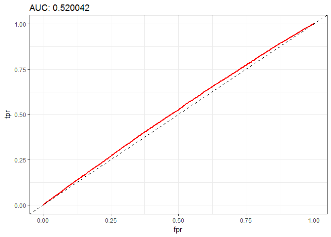
model_performance(linear_model)
h2o.confusionMatrix(linear_model, newdata = h_test)

## Confusion Matrix for max f1 @ threshold = 0.448915207674831:
##         DIRE RADIANT    Error          Rate
## DIRE       3   48136 0.999938  =48136/48139
## RADIANT    1   51860 0.000019      =1/51861
## Totals     4   99996 0.481370  =48137/1e+05
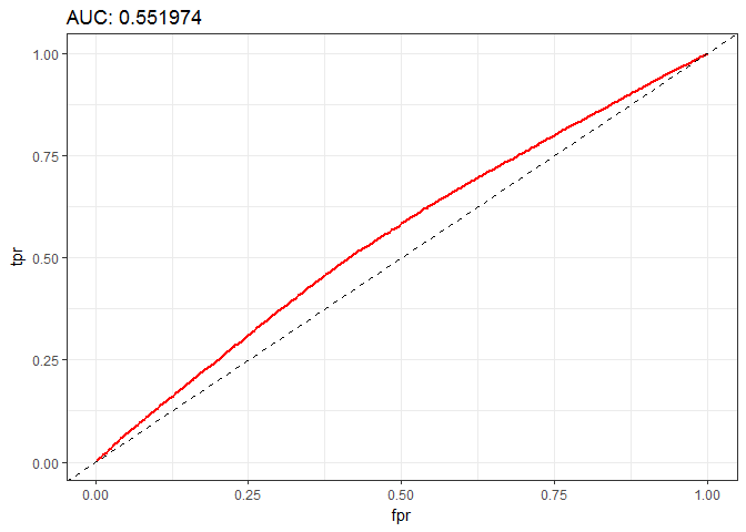
Ok. It is only a slight better than pure guessing. From my own playing experience I know that in this game playing more matches are very important. Adding this kind of information as a feature may have a positive effect on the guessing.
In the second experiment the number of total matches the players played will be added as feature alongside with the averages too.
# In player ratings for account 0 (all of unidentified accounts) the number of matches are not for one player but all of the unidentified players. Also there are missing values. This will be corrected to use an average.
avg_legacy_match_count <- as.integer(round(mean(as.numeric(legacy_player_ratings[legacy_player_ratings$account_id != 0, "total_matches"]$total_matches))))
legacy_player_ratings[legacy_player_ratings$account_id == 0 | is.na(legacy_player_ratings$account_id), "total_matches"] <- avg_legacy_match_count

# Distribution of value:
p1 <- ggplot(data = legacy_player_ratings) + geom_histogram(aes(x = total_matches))
p2 <- ggplot(data = legacy_player_ratings) + geom_histogram(aes(x = log(total_matches)))

grid.arrange(p1, p2, ncol=2, top = "Distribution of total_matches")
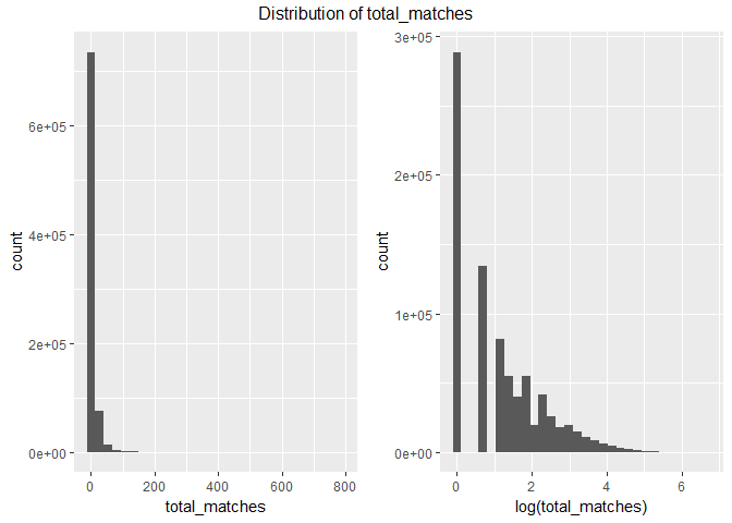 According to the histograms taking logs is a good idea in this case. The
distribution is still far from Gaussian but looks more usable.
feature2 <- function(legacy_player_ratings, players, feature1, avg_legacy_match_count) {
  playerdata <- data.table(left_join(players_train, legacy_player_ratings[,.(account_id, total_matches)], by = "account_id"))
  playerdata[is.na(total_matches), total_matches:=avg_legacy_match_count]

  # player_slot 0-4: radiant, 128-132: dire
  playerdata[, side:= as.factor(if_else(player_slot < 100, true = "RADIANT", false = "DIRE"))]

  teamstat <- playerdata %>% group_by(match_id, side) %>% summarise(ln_avg_matches_legacy=log(mean(total_matches)), ln_total_matches_legacy=log(sum(total_matches)))

  teamstat_join_columns <- c("match_id", "ln_avg_matches_legacy", "ln_total_matches_legacy")
  teamstat <- left_join(teamstat[teamstat$side == "RADIANT", teamstat_join_columns],
                  teamstat[teamstat$side == "DIRE", teamstat_join_columns],
                  by="match_id", suffix=c("_RADIANT", "_DIRE")
              )
  out <- left_join(feature1, teamstat, by="match_id")

  return(out)
}

train <- feature2(legacy_player_ratings, players_train, train, avg_legacy_match_count)
test <- feature2(legacy_player_ratings, players_test, test, avg_legacy_match_count)


upload_data(train, test)

linear_model <- h2o.glm(x = c(
  "win_percent_legacy_RADIANT",
  "win_percent_legacy_DIRE",
  "ln_avg_matches_legacy_RADIANT",
  "ln_avg_matches_legacy_DIRE",
  "ln_total_matches_legacy_RADIANT",
  "ln_total_matches_legacy_DIRE"),
  y = "winner",
  training_frame = h_train, validation_frame = h_test,
  family = "binomial",
  score_each_iteration = TRUE)

model_performance(linear_model)
h2o.confusionMatrix(linear_model, newdata = h_test)

## Confusion Matrix for max f1 @ threshold = 0.471339903330327:
##         DIRE RADIANT    Error          Rate
## DIRE       3   48136 0.999938  =48136/48139
## RADIANT    1   51860 0.000019      =1/51861
## Totals     4   99996 0.481370  =48137/1e+05
Unfortunately the prediction accuracy didn't increase. We have to find new ways to improve the accuracy.
Actually the real game begins at character selection. A good combination of the heroes can lead to victory even for weaker players too. All the heroes will be added as a binary indicator variable. (Hero ids: [1, 113])
As the linear model starting to become more complicated a random forest model will be evaluated too. Random forest can provide a good output with minimal effort and it is resilient to over-fitting.
feature3 <- function(players, feature2) {
  herodata <- players[, list(match_id, player_slot, hero_id)]
  melted <- melt(herodata, id.vars = c("match_id", "player_slot"))
  melted[, variable:=as.factor(paste(ifelse(player_slot < 100, "RADIANT", "DIRE"), "hero", value, sep = "_"))]
  melted[, value:=1]
  herodata <- dcast(melted, match_id ~ variable)

  out <- left_join(feature2, herodata, by="match_id")

  return(out)
}

train <- feature3(players_train, train)
test <- feature3(players_test, test)

upload_data(train, test)

linear_model <- h2o.glm(
  x = colnames(train)[3:length(colnames(train))],
  y = "winner",
  training_frame = h_train, validation_frame = h_test,
  family = "binomial",
  score_each_iteration = TRUE)

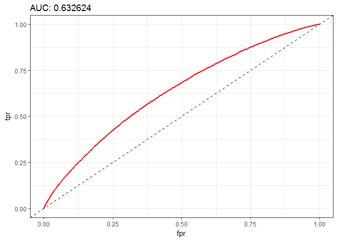
model_performance(linear_model)
h2o.confusionMatrix(linear_model, newdata = h_test)

## Confusion Matrix for max f1 @ threshold = 0.338317623250638:
##         DIRE RADIANT    Error          Rate
## DIRE    4303   43836 0.910613  =43836/48139
## RADIANT 1808   50053 0.034862   =1808/51861
## Totals  6111   93889 0.456440  =45644/1e+05

random_forest <- h2o.randomForest(
  x = colnames(train)[3:length(colnames(train))],
  y = "winner",
  training_frame = h_train, validation_frame = h_test
  # score_each_iteration = TRUE
  )

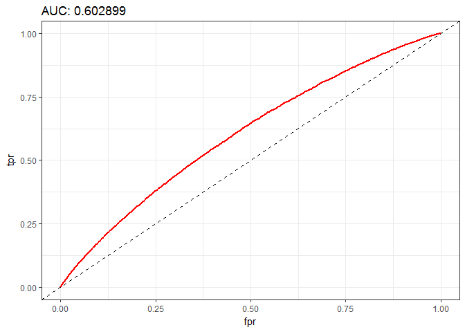
model_performance(random_forest)
h2o.confusionMatrix(random_forest, newdata = h_test)

## Confusion Matrix for max f1 @ threshold = 0.413738227358363:
##         DIRE RADIANT    Error          Rate
## DIRE    1764   46375 0.963356  =46375/48139
## RADIANT  783   51078 0.015098    =783/51861
## Totals  2547   97453 0.471580  =47158/1e+05
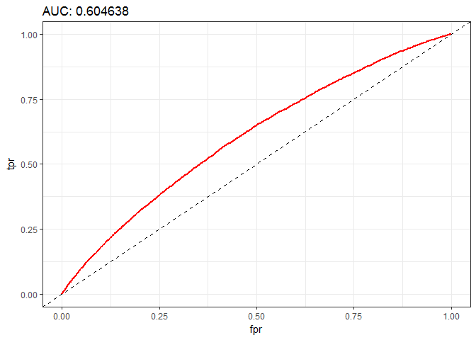
The theory was confirmed: Adding information of hero selection increased the AUX about 11 percentage points for linear model. Random forest didn't performed that well as the linear model but using the new features it was still better than the linear model previously.
The following player stats will be calculated from ranked match data to have a detailed information regarding the individual player skill:
-
Kill death ratio (kdr) : An important statistics that shows the players skill. Unfortunately only killing blows count as kills therefore this ratio will be adjusted by counting assists (when the player participated in the kill but an other player got the actual kill)
-
Average XP/min : Higher value means that the player participated in fights more actively and by acquiring more experience points he could level up faster. Level advantage is a decision maker between win/lose.
-
Average Gold/min : Higher value means that the player was able to have more lat hits (That earns golds) or was able to destroy enemy structures. With more gold the player could buy more advanced items and this is improving his team's chance to win.
These player performance indicators will be assigned to the corresponding player slot instead using simple averages. As an expectation it will add better control for players with exceptional skills because this kind of players can carry the match and win it. As usual account_id 0 is for unidentified players. The average values of all unidentified players imputed here.
player_stat_rated <- players_train %>% group_by(account_id) %>%
  summarise(kdr=(sum(kills)+sum(assists))/sum(deaths), avg_xp_per_min=mean(xp_per_min), avg_gold_per_min=mean(gold_per_min))

# Distribution of values:
distplot <- function(dat, label_prefix) {
  p1 <- ggplot(data = dat) + geom_histogram(aes(x = kdr)) + xlab(paste(label_prefix, "kdr", sep = ""))
  p2 <- ggplot(data = dat) + geom_histogram(aes(x = avg_xp_per_min)) + xlab(paste(label_prefix, "avg_xp_per_min", sep = ""))
  p3 <- ggplot(data = dat) + geom_histogram(aes(x = avg_gold_per_min)) + xlab(paste(label_prefix, "avg_gold_per_min", sep = ""))

  grid.arrange(p1, p2, p3, ncol = 3, top = "Distribution of values")
}

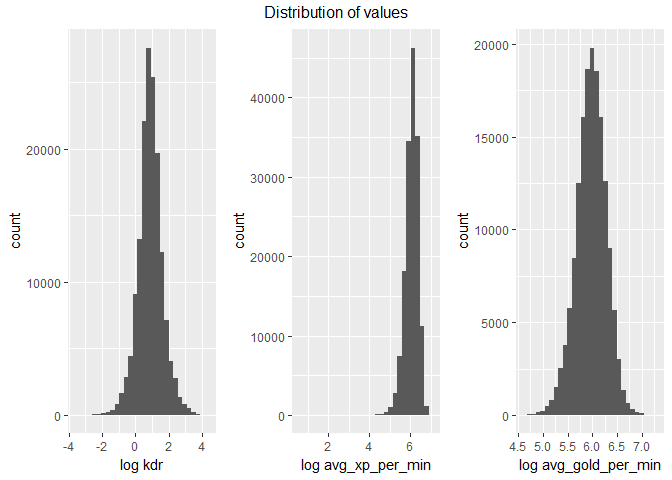
distplot(player_stat_rated, "")
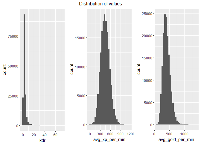 Kdr and avg_gold_per_min shows a right tail and also we are going for
differences here rather than levels thus taking logs should be
beneficial.
player_stat_rated$kdr <- log(player_stat_rated$kdr)
player_stat_rated$avg_xp_per_min <- log(player_stat_rated$avg_xp_per_min)
player_stat_rated$avg_gold_per_min <- log(player_stat_rated$avg_gold_per_min)

distplot(player_stat_rated, "log ")
feature4 <- function(players, feature3) {
  herodata <- players[, list(match_id, player_slot, account_id)]
  melted <- melt(herodata, id.vars = c("match_id", "player_slot"))
  melted <- data.table(left_join(melted, player_stat_rated, by=c("value" = "account_id")))
  melted[, variable:=as.factor(paste(ifelse(player_slot < 100, "RADIANT", "DIRE"), "kdr", player_slot %% 128, sep = "_"))]
  melted$value <- melted$kdr
  herodata1 <- dcast(melted, match_id ~ variable)
  melted[, variable:=as.factor(paste(ifelse(player_slot < 100, "RADIANT", "DIRE"), "avg_xp_per_min", player_slot %% 128, sep = "_"))]
  melted$value <- melted$avg_xp_per_min
  herodata2 <- dcast(melted, match_id ~ variable)
  melted[, variable:=as.factor(paste(ifelse(player_slot < 100, "RADIANT", "DIRE"), "avg_gold_per_min", player_slot %% 128, sep = "_"))]
  melted$value <- melted$avg_gold_per_min
  herodata3 <- dcast(melted, match_id ~ variable)

  herodata <- left_join(herodata1, herodata2, by="match_id")
  herodata <- left_join(herodata, herodata3, by="match_id")

  out <- left_join(feature3, herodata, by="match_id")

  return(out)
}

train_2 <- feature4(players_train, train)
test_2 <- feature4(players_test, test)

upload_data(train_2, test_2)

linear_model <- h2o.glm(
  x = colnames(train_2)[3:length(colnames(train_2))],
  y = "winner",
  training_frame = h_train, validation_frame = h_test,
  family = "binomial",
  score_each_iteration = TRUE)

model_performance(linear_model)
h2o.confusionMatrix(linear_model, newdata = h_test)

## Confusion Matrix for max f1 @ threshold = 0.00117918782384543:
##         DIRE RADIANT    Error          Rate
## DIRE       0   48139 1.000000  =48139/48139
## RADIANT    0   51861 0.000000      =0/51861
## Totals     0  100000 0.481390  =48139/1e+05

gb_model <- h2o.gbm(
  x = colnames(train)[3:length(colnames(train))],
  y = "winner",
  training_frame = h_train, validation_frame = h_test,
  score_each_iteration = TRUE)

model_performance(gb_model)
h2o.confusionMatrix(gb_model, newdata = h_test)

## Confusion Matrix for max f1 @ threshold = 0.417290973476894:
##         DIRE RADIANT    Error          Rate
## DIRE    2655   45484 0.944847  =45484/48139
## RADIANT 1268   50593 0.024450   =1268/51861
## Totals  3923   96077 0.467520  =46752/1e+05
The AUC became worse by adding these features. It looks like the model is starting to became more complicated and it is starting to overfit. The previous feature set will be used for final evaluation. (Experiment 3)
Several different model with different parameters (GBM, Random Forest, Neural Network) have been tested using the H_2_O Flow UI but neither of them provided the accuracy of the linear model used in Experiment 3: Experiment 3 results:
upload_data(train, test)


linear_model <- h2o.glm(
  x = colnames(train)[3:length(colnames(train))],
  y = "winner",
  training_frame = h_train, validation_frame = h_test,
  family = "binomial",
  score_each_iteration = TRUE)

model_performance(linear_model)
h2o.confusionMatrix(linear_model, newdata = h_test)

## Confusion Matrix for max f1 @ threshold = 0.338317623250638:
##         DIRE RADIANT    Error          Rate
## DIRE    4303   43836 0.910613  =43836/48139
## RADIANT 1808   50053 0.034862   =1808/51861
## Totals  6111   93889 0.456440  =45644/1e+05
The final accuracy is 63% what is much better than random guessing and it is a pretty good result considering the fact that the matches organized by a ranking system that tryes to assign teams with similar skill levels to a match.
colnames(train)

##   [1] "match_id"                        "winner"
##   [3] "win_percent_legacy_RADIANT"      "win_percent_legacy_DIRE"
##   [5] "ln_avg_matches_legacy_RADIANT"   "ln_total_matches_legacy_RADIANT"
##   [7] "ln_avg_matches_legacy_DIRE"      "ln_total_matches_legacy_DIRE"
##   [9] "DIRE_hero_0"                     "DIRE_hero_1"
##  [11] "DIRE_hero_10"                    "DIRE_hero_100"
##  [13] "DIRE_hero_101"                   "DIRE_hero_102"
##  [15] "DIRE_hero_103"                   "DIRE_hero_104"
##  [17] "DIRE_hero_105"                   "DIRE_hero_106"
##  [19] "DIRE_hero_107"                   "DIRE_hero_109"
##  [21] "DIRE_hero_11"                    "DIRE_hero_110"
##  [23] "DIRE_hero_111"                   "DIRE_hero_112"
##  [25] "DIRE_hero_12"                    "DIRE_hero_13"
##  [27] "DIRE_hero_14"                    "DIRE_hero_15"
##  [29] "DIRE_hero_16"                    "DIRE_hero_17"
##  [31] "DIRE_hero_18"                    "DIRE_hero_19"
##  [33] "DIRE_hero_2"                     "DIRE_hero_20"
##  [35] "DIRE_hero_21"                    "DIRE_hero_22"
##  [37] "DIRE_hero_23"                    "DIRE_hero_25"
##  [39] "DIRE_hero_26"                    "DIRE_hero_27"
##  [41] "DIRE_hero_28"                    "DIRE_hero_29"
##  [43] "DIRE_hero_3"                     "DIRE_hero_30"
##  [45] "DIRE_hero_31"                    "DIRE_hero_32"
##  [47] "DIRE_hero_33"                    "DIRE_hero_34"
##  [49] "DIRE_hero_35"                    "DIRE_hero_36"
##  [51] "DIRE_hero_37"                    "DIRE_hero_38"
##  [53] "DIRE_hero_39"                    "DIRE_hero_4"
##  [55] "DIRE_hero_40"                    "DIRE_hero_41"
##  [57] "DIRE_hero_42"                    "DIRE_hero_43"
##  [59] "DIRE_hero_44"                    "DIRE_hero_45"
##  [61] "DIRE_hero_46"                    "DIRE_hero_47"
##  [63] "DIRE_hero_48"                    "DIRE_hero_49"
##  [65] "DIRE_hero_5"                     "DIRE_hero_50"
##  [67] "DIRE_hero_51"                    "DIRE_hero_52"
##  [69] "DIRE_hero_53"                    "DIRE_hero_54"
##  [71] "DIRE_hero_55"                    "DIRE_hero_56"
##  [73] "DIRE_hero_57"                    "DIRE_hero_58"
##  [75] "DIRE_hero_59"                    "DIRE_hero_6"
##  [77] "DIRE_hero_60"                    "DIRE_hero_61"
##  [79] "DIRE_hero_62"                    "DIRE_hero_63"
##  [81] "DIRE_hero_64"                    "DIRE_hero_65"
##  [83] "DIRE_hero_66"                    "DIRE_hero_67"
##  [85] "DIRE_hero_68"                    "DIRE_hero_69"
##  [87] "DIRE_hero_7"                     "DIRE_hero_70"
##  [89] "DIRE_hero_71"                    "DIRE_hero_72"
##  [91] "DIRE_hero_73"                    "DIRE_hero_74"
##  [93] "DIRE_hero_75"                    "DIRE_hero_76"
##  [95] "DIRE_hero_77"                    "DIRE_hero_78"
##  [97] "DIRE_hero_79"                    "DIRE_hero_8"
##  [99] "DIRE_hero_80"                    "DIRE_hero_81"
## [101] "DIRE_hero_82"                    "DIRE_hero_83"
## [103] "DIRE_hero_84"                    "DIRE_hero_85"
## [105] "DIRE_hero_86"                    "DIRE_hero_87"
## [107] "DIRE_hero_88"                    "DIRE_hero_89"
## [109] "DIRE_hero_9"                     "DIRE_hero_90"
## [111] "DIRE_hero_91"                    "DIRE_hero_92"
## [113] "DIRE_hero_93"                    "DIRE_hero_94"
## [115] "DIRE_hero_95"                    "DIRE_hero_96"
## [117] "DIRE_hero_97"                    "DIRE_hero_98"
## [119] "DIRE_hero_99"                    "RADIANT_hero_0"
## [121] "RADIANT_hero_1"                  "RADIANT_hero_10"
## [123] "RADIANT_hero_100"                "RADIANT_hero_101"
## [125] "RADIANT_hero_102"                "RADIANT_hero_103"
## [127] "RADIANT_hero_104"                "RADIANT_hero_105"
## [129] "RADIANT_hero_106"                "RADIANT_hero_107"
## [131] "RADIANT_hero_109"                "RADIANT_hero_11"
## [133] "RADIANT_hero_110"                "RADIANT_hero_111"
## [135] "RADIANT_hero_112"                "RADIANT_hero_12"
## [137] "RADIANT_hero_13"                 "RADIANT_hero_14"
## [139] "RADIANT_hero_15"                 "RADIANT_hero_16"
## [141] "RADIANT_hero_17"                 "RADIANT_hero_18"
## [143] "RADIANT_hero_19"                 "RADIANT_hero_2"
## [145] "RADIANT_hero_20"                 "RADIANT_hero_21"
## [147] "RADIANT_hero_22"                 "RADIANT_hero_23"
## [149] "RADIANT_hero_25"                 "RADIANT_hero_26"
## [151] "RADIANT_hero_27"                 "RADIANT_hero_28"
## [153] "RADIANT_hero_29"                 "RADIANT_hero_3"
## [155] "RADIANT_hero_30"                 "RADIANT_hero_31"
## [157] "RADIANT_hero_32"                 "RADIANT_hero_33"
## [159] "RADIANT_hero_34"                 "RADIANT_hero_35"
## [161] "RADIANT_hero_36"                 "RADIANT_hero_37"
## [163] "RADIANT_hero_38"                 "RADIANT_hero_39"
## [165] "RADIANT_hero_4"                  "RADIANT_hero_40"
## [167] "RADIANT_hero_41"                 "RADIANT_hero_42"
## [169] "RADIANT_hero_43"                 "RADIANT_hero_44"
## [171] "RADIANT_hero_45"                 "RADIANT_hero_46"
## [173] "RADIANT_hero_47"                 "RADIANT_hero_48"
## [175] "RADIANT_hero_49"                 "RADIANT_hero_5"
## [177] "RADIANT_hero_50"                 "RADIANT_hero_51"
## [179] "RADIANT_hero_52"                 "RADIANT_hero_53"
## [181] "RADIANT_hero_54"                 "RADIANT_hero_55"
## [183] "RADIANT_hero_56"                 "RADIANT_hero_57"
## [185] "RADIANT_hero_58"                 "RADIANT_hero_59"
## [187] "RADIANT_hero_6"                  "RADIANT_hero_60"
## [189] "RADIANT_hero_61"                 "RADIANT_hero_62"
## [191] "RADIANT_hero_63"                 "RADIANT_hero_64"
## [193] "RADIANT_hero_65"                 "RADIANT_hero_66"
## [195] "RADIANT_hero_67"                 "RADIANT_hero_68"
## [197] "RADIANT_hero_69"                 "RADIANT_hero_7"
## [199] "RADIANT_hero_70"                 "RADIANT_hero_71"
## [201] "RADIANT_hero_72"                 "RADIANT_hero_73"
## [203] "RADIANT_hero_74"                 "RADIANT_hero_75"
## [205] "RADIANT_hero_76"                 "RADIANT_hero_77"
## [207] "RADIANT_hero_78"                 "RADIANT_hero_79"
## [209] "RADIANT_hero_8"                  "RADIANT_hero_80"
## [211] "RADIANT_hero_81"                 "RADIANT_hero_82"
## [213] "RADIANT_hero_83"                 "RADIANT_hero_84"
## [215] "RADIANT_hero_85"                 "RADIANT_hero_86"
## [217] "RADIANT_hero_87"                 "RADIANT_hero_88"
## [219] "RADIANT_hero_89"                 "RADIANT_hero_9"
## [221] "RADIANT_hero_90"                 "RADIANT_hero_91"
## [223] "RADIANT_hero_92"                 "RADIANT_hero_93"
## [225] "RADIANT_hero_94"                 "RADIANT_hero_95"
## [227] "RADIANT_hero_96"                 "RADIANT_hero_97"
## [229] "RADIANT_hero_98"                 "RADIANT_hero_99"
