A python library for creating cobweb plots, bifurcation diagrams, and calculating the Lyapunov exponents of one-dimensional maps.
The library includes several common one-dimensional maps and discrete-time evolutionary/learning dynamics such as the replicator dynamic.
When calculating Lyapunov exponents you can either pass the map's first-order derivative, or the plotting function can calculate the derivative using scipy.misc.derivative. Unfortunately, scipy's derivate function can be very slow and may raise errors depending on the map's shape.
To create a bifurcation diagram paired with Lyapunov exponents for the sine map...
import numpy as np
import chaotic_maps as cm

cm.bifurcation_and_lyapunov_plots(
    cm.sin_map,
    init=0.2,
    parameter_range=np.linspace(0.6, 1, num=10000),
    deriv_generator=cm.sin_map_deriv,
    y_points=500,
    xlabel=r"$\mu$",
    ylabel=r"$x$",
    file_name="sine.png",
)
The package can generate whole plots, or you can feed it axes to populate. For example, the following will show two bifurcation diagrams fror the Gauss Iterated Map side-by-side...
import numpy as np
import matplotlib.pyplot as plt
import chaotic_maps as cm

fig, axes = plt.subplots(1,2, figsize=(12,5))

cm.bifurcation_plot(
    cm.gauss_map_family(alpha=5),
    init=0.1,
    parameter_range=np.linspace(-0.9, 1, 10000),
    y_points=500,
    xlabel=r"$\beta$",
    ylabel=r"$x$",
    set_title=r"$\alpha = 5$",
    ax=axes[0]
)

cm.bifurcation_plot(
    cm.gauss_map_family(alpha=6.5),
    init=0.1,
    parameter_range=np.linspace(-0.9, 1, 10000),
    y_points=500,
    xlabel=r"$\beta$",
    ylabel=r"$x$",
    set_title=r"$\alpha = 6.5$",
    ax=axes[1]
)

plt.savefig("gauss.png", dpi=300)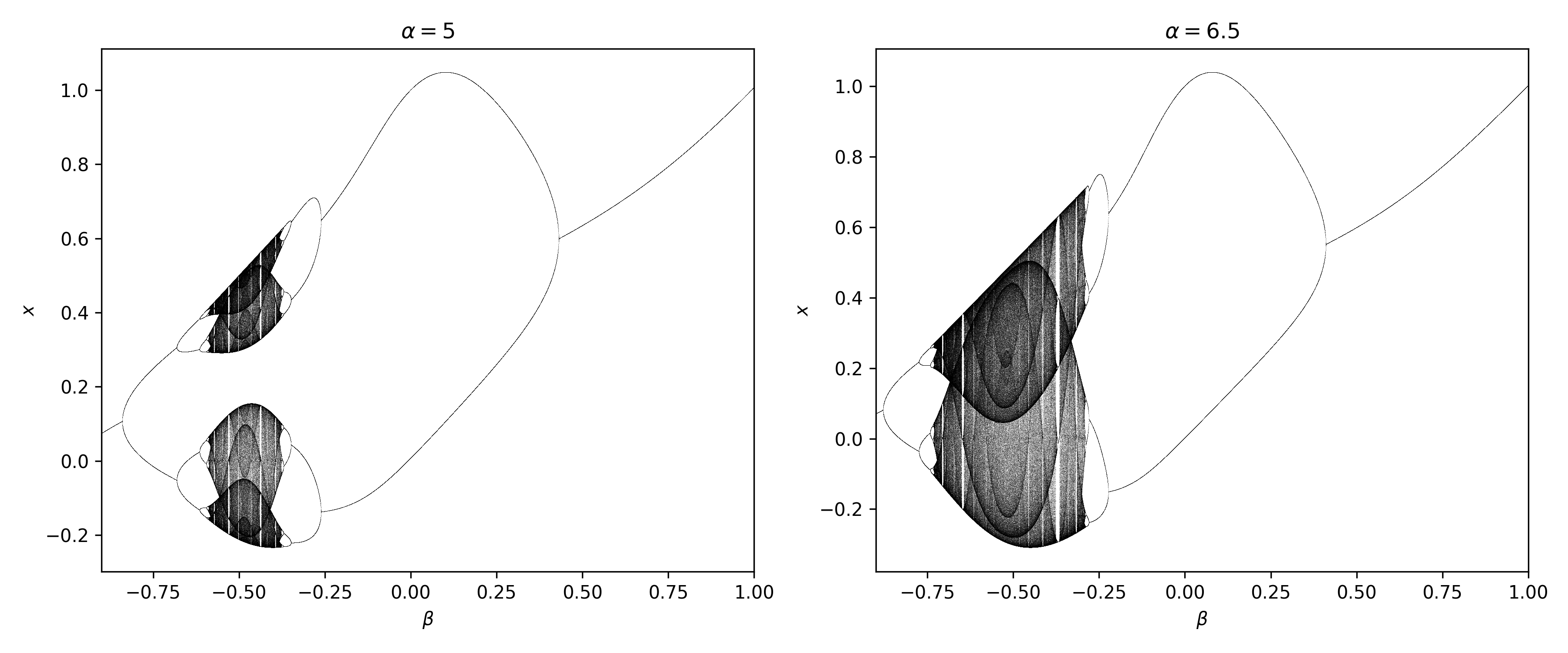
You can also use chaotic_maps to create cobweb plots. Here are four cobweb plots for the Sine map showing long-run behavior under different parameters.
import numpy as np
import matplotlib.pyplot as plt
import chaotic_maps as cm

fig, axes = plt.subplots(2, 2)

cm.cobweb_plot(cm.sin_map(.7), .1, 50, domain=np.linspace(0, 1), ax=axes[0][0], ylabel=r'$x_{n+1}$')
cm.cobweb_plot(cm.sin_map(.8), .1, 10, domain=np.linspace(0, 1), ax=axes[0][1])
cm.cobweb_plot(cm.sin_map(.85), .1, 50, domain=np.linspace(0, 1), ax=axes[1][0], xlabel=r'$x_n$', ylabel=r'$x_{n+1}$')
cm.cobweb_plot(cm.sin_map(.9), .1, 150, domain=np.linspace(0, 1), ax=axes[1][1], xlabel=r'$x_n$')

axes[0][0].set_title(r'$\mu = 0.7$')
axes[0][1].set_title(r'$\mu = 0.8$')
axes[1][0].set_title(r'$\mu = 0.85$')
axes[1][1].set_title(r'$\mu = 0.9$')

plt.tight_layout()
plt.savefig("sin_cobwebs.png", dpi=300)