This notebook is available on: https://github.com/epspi/02.28.2017_Cin-Day_RUG_sparklyr
The data is available at census.gov: https://www.census.gov/econ/cfs/pums.html
A fully instructive tutorial is at: http://spark.rstudio.com/
sparklyr and dplyr is what we'll be using. Install Spark directly from R with the handy spark_install() function within sparklyr
if (!require(dplyr)) install.packages("dplyr")
if (!require(data.table)) install.packages("data.table")
if (!require(sparklyr)) install.packages("sparklyr")library(dplyr)
library(data.table)
library(sparklyr)
# spark_install(version = "2.0.1")
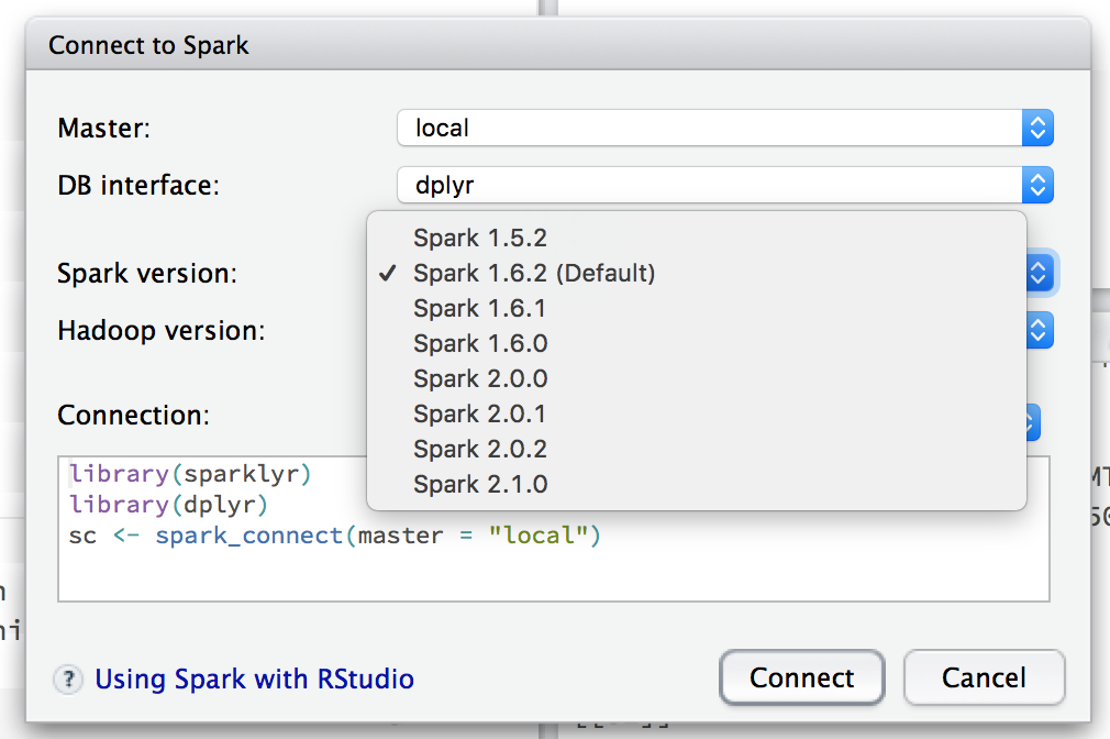
# spark_install(version = "1.6.2")You can connect to spark using the GUI or by calling spark_connect and specifying which version of Spark you want to use and whether you want a local or remote master. If you don't specify a version, it will default to version 1.6.2 (as of March 2017).
sc <- spark_connect(master = "local", version = "2.0.1")

# If you have port conflicts, try:
# config <- spark_config()
# config$sparklyr.gateway.port <-  5454
# sc <- spark_connect(master = "local", config = config)

sc
## $master
## [1] "local[4]"
##
## $method
## [1] "shell"
##
## $app_name
## [1] "sparklyr"
##
## $config
## $config$sparklyr.cores.local
## [1] 4
##
## $config$spark.sql.shuffle.partitions.local
## [1] 4
##
## $config$spark.env.SPARK_LOCAL_IP.local
## [1] "127.0.0.1"
##
## $config$sparklyr.csv.embedded
...
# List of RDDs currently in the cluster
src_tbls(sc)
# Web utility
spark_web(sc)We need to feed data into the Spark cluster, whether by copying it from R objects or by using one of the filereader functions.
# Read in the text file locally and then copy_to Spark
system.time({
    ship <- fread("data/cfs_2012_pumf_csv.txt")
    ship_sp <- copy_to(sc, ship, "ship", overwrite = T)
})
##
Read 4547661 rows and 20 (of 20) columns from 0.350 GB file in 00:00:06
##    user  system elapsed
##  52.058   3.485  80.862
# src_tbls(sc)There are (at least) three readers for getting data directly into the cluster:
spark_read_csvspark_read_parquetspark_read_json
system.time(
    ship2_sp <- spark_read_csv(sc, "ship2",
                           "data/cfs_2012_pumf_csv.txt")
)
## user system elapsed
## 0.042 0.003 31.251
We can't use names to figure out what's in the spark tables,
but colnames and tbl_vars work
# colnames(ship_sp)
tbl_vars(ship2_sp)
## [1] "SHIPMT_ID" "ORIG_STATE" "ORIG_MA"
## [4] "ORIG_CFS_AREA" "DEST_STATE" "DEST_MA"
## [7] "DEST_CFS_AREA" "NAICS" "QUARTER"
## [10] "SCTG" "MODE" "SHIPMT_VALUE"
## [13] "SHIPMT_WGHT" "SHIPMT_DIST_GC" "SHIPMT_DIST_ROUTED"
## [16] "TEMP_CNTL_YN" "EXPORT_YN" "EXPORT_CNTRY"
## [19] "HAZMAT" "WGT_FACTOR"
The RStudio table viewer also works on Spark tables
head(ship2_sp) %>% ViewYou can use some (all?) of the dplyr verbs and also SQL commands directly on spark tables. That's basically the whole point.
ship2_sp %>% count(ORIG_STATE)## Source: query [52 x 2]
## Database: spark connection master=local[4] app=sparklyr local=TRUE
##
## ORIG_STATE n
## <int> <dbl>
## 1 25 97933
## 2 12 172342
## 3 13 130663
## 4 37 148681
## 5 18 141060
## 6 38 23188
## 7 56 15868
## 8 46 31072
## 9 50 22781
## 10 42 205959
## # ... with 42 more rows
Spark will defer calculation until you deliberately or implictely try to collect the data back as an R object.
head(ship2_sp)## Source: query [6 x 20]
## Database: spark connection master=local[4] app=sparklyr local=TRUE
##
## SHIPMT_ID ORIG_STATE ORIG_MA ORIG_CFS_AREA DEST_STATE DEST_MA
## <int> <int> <int> <chr> <int> <int>
## 1 1 25 148 25-148 25 148
## 2 2 42 428 42-428 6 41740
## 3 3 26 220 26-220 47 314
## 4 4 20 556 20-556 20 556
## 5 5 12 99999 12-99999 12 99999
## 6 6 24 47900 24-47900 30 99999
## # ... with 14 more variables: DEST_CFS_AREA <chr>, NAICS <int>,
## # QUARTER <int>, SCTG <chr>, MODE <int>, SHIPMT_VALUE <int>,
## # SHIPMT_WGHT <int>, SHIPMT_DIST_GC <int>, SHIPMT_DIST_ROUTED <int>,
## # TEMP_CNTL_YN <chr>, EXPORT_YN <chr>, EXPORT_CNTRY <chr>, HAZMAT <chr>,
## # WGT_FACTOR <dbl>
spark_log(sc, n = 3)## 17/03/15 22:20:04 INFO TaskSchedulerImpl: Removed TaskSet 30.0, whose tasks have all completed, from pool
## 17/03/15 22:20:04 INFO DAGScheduler: ResultStage 30 (collect at utils.scala:195) finished in 0.009 s
## 17/03/15 22:20:04 INFO DAGScheduler: Job 18 finished: collect at utils.scala:195, took 0.015261 s
For example, we select some columns of interest and assign the resulting df to a new variables. However, as we see by calling names or str on the resulting variable, it's still a spark object, not a collected df.
ship_values <- ship2_sp %>%
    select(contains("SHIPMT"))

names(ship_values)
## [1] "src" "ops"
Once we ask for the contents of ship_values, however, an implicit collection occurs
ship_values %>% head## Source: query [6 x 5]
## Database: spark connection master=local[4] app=sparklyr local=TRUE
##
## SHIPMT_ID SHIPMT_VALUE SHIPMT_WGHT SHIPMT_DIST_GC SHIPMT_DIST_ROUTED
## <int> <int> <int> <int> <int>
## 1 1 2178 11 14 17
## 2 2 344 11 2344 2734
## 3 3 4197 5134 470 579
## 4 4 116 6 3 3
## 5 5 388 527 124 201
## 6 6 3716 1132 1942 2265
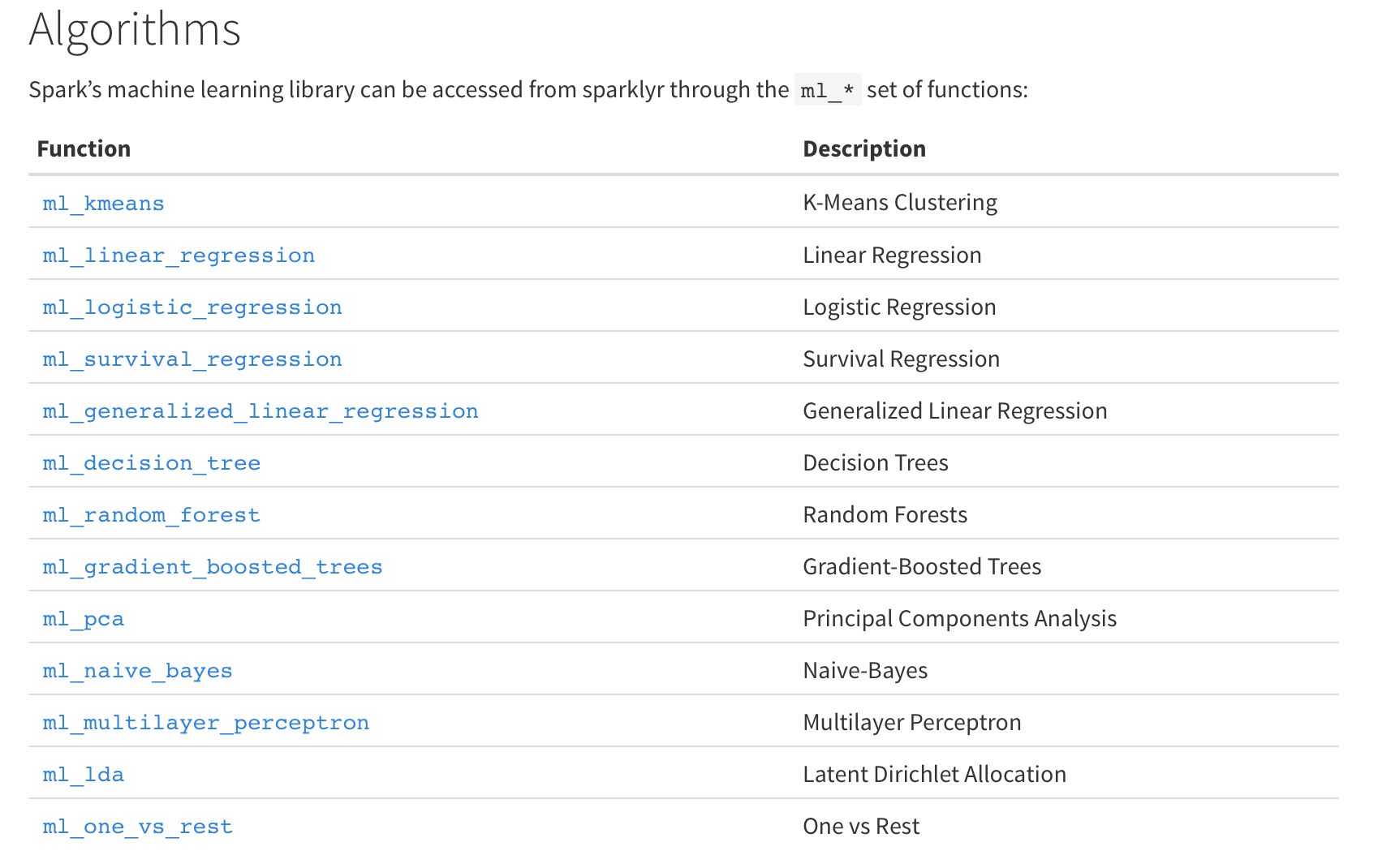
The sparklyr API includes interfaces to way more Spark ML facilities than the previous API from Spark directly.
Let's try running a simple linear regression of shipment values of some other numeric variables
system.time({
    lm_sp <- ship_values %>%
    select(-SHIPMT_ID) %>%
    ml_linear_regression(SHIPMT_VALUE ~ .)
})
## * No rows dropped by 'na.omit' call
##    user  system elapsed
##   0.084   0.005  14.550
system.time({
    dat <- ship %>%
    select(contains("SHIPMT")) %>%
    select(-SHIPMT_ID)

lm_R <- lm(SHIPMT_VALUE ~ ., data = dat)
})
## user system elapsed
## 8.072 1.079 9.758
The output of the Spark linear regression is an object of a different type than the usual lm class.
class(lm_sp)## [1] "ml_model_linear_regression" "ml_model"
class(lm_R)## [1] "lm"
##
## Spark LM Summary Output
summary(lm_sp)## Call: ml_linear_regression(., SHIPMT_VALUE ~ .)
##
## Deviance Residuals: (approximate):
## Min 1Q Median 3Q Max
## -11584891 -13220 -12181 -8894 521254508
##
## Coefficients:
## Estimate Std. Error t value Pr(>|t|)
## (Intercept) 1.2402e+04 6.1687e+02 20.1046 < 2.2e-16 ***
## SHIPMT_WGHT 1.1866e-01 5.2415e-04 226.3765 < 2.2e-16 ***
## SHIPMT_DIST_GC -3.5101e+01 5.9366e+00 -5.9127 3.366e-09 ***
## SHIPMT_DIST_ROUTED 3.1517e+01 4.9665e+00 6.3459 2.212e-10 ***
## ---
## Signif. codes: 0 '***' 0.001 '**' 0.01 '*' 0.05 '.' 0.1 ' ' 1
##
## R-Squared: 0.01118
## Root Mean Squared Error: 1079000
##
## R LM Summary Output
summary(lm_R)##
## Call:
## lm(formula = SHIPMT_VALUE ~ ., data = dat)
##
## Residuals:
## Min 1Q Median 3Q Max
## -32276343 -13209 -12181 -8893 521254508
##
## Coefficients:
## Estimate Std. Error t value Pr(>|t|)
## (Intercept) 1.240e+04 6.169e+02 20.105 < 2e-16 ***
## SHIPMT_WGHT 1.187e-01 5.242e-04 226.377 < 2e-16 ***
## SHIPMT_DIST_GC -3.510e+01 5.937e+00 -5.913 3.37e-09 ***
## SHIPMT_DIST_ROUTED 3.152e+01 4.966e+00 6.346 2.21e-10 ***
## ---
## Signif. codes: 0 '***' 0.001 '**' 0.01 '*' 0.05 '.' 0.1 ' ' 1
##
## Residual standard error: 1079000 on 4547657 degrees of freedom
## Multiple R-squared: 0.01118, Adjusted R-squared: 0.01117
## F-statistic: 1.713e+04 on 3 and 4547657 DF, p-value: < 2.2e-16
The Spark machine learning output object has basically all the same values as the equivalent R object
names(lm_sp)## [1] "features" "response"
## [3] "intercept" "coefficients"
## [5] "standard.errors" "t.values"
## [7] "p.values" "explained.variance"
## [9] "mean.absolute.error" "mean.squared.error"
## [11] "r.squared" "root.mean.squared.error"
## [13] "data" "ml.options"
## [15] "categorical.transformations" "model.parameters"
## [17] ".call" ".model"
One difference is that the Spark output does not contain the original data (for good reason!), which means that there is no plot method defined on the object.
# DOES NOT WORK!
#plot(lm_sp)

# Works but may crash anyways due to size
#plot(lm_R)Let's split the dataset according to origin state (ORIG_STATE) and fit a linear model to each subset.
system.time({
    stateModelsR <- ship %>%
        select(ORIG_STATE, contains("SHIPMT"), -SHIPMT_ID) %>%
        by(., .$ORIG_STATE, . %>% {
            lm(SHIPMT_VALUE ~ . - ORIG_STATE, data = .)
        })
})
## user system elapsed
## 9.184 1.792 11.759
stateModelsR## .$ORIG_STATE: 0
##
## Call:
## lm(formula = SHIPMT_VALUE ~ . - ORIG_STATE, data = .)
##
## Coefficients:
## (Intercept) SHIPMT_WGHT SHIPMT_DIST_GC
## 3455.4317 0.2394 8.9563
## SHIPMT_DIST_ROUTED
## -4.0085
##
## --------------------------------------------------------
## .$ORIG_STATE: 1
##
## Call:
## lm(formula = SHIPMT_VALUE ~ . - ORIG_STATE, data = .)
##
## Coefficients:
## (Intercept) SHIPMT_WGHT SHIPMT_DIST_GC
## 8560.56310 0.08376 -63.52657
## SHIPMT_DIST_ROUTED
## 60.38119
##
## --------------------------------------------------------
##
## ... etc
##
## --------------------------------------------------------
## .$ORIG_STATE: 56
##
## Call:
## lm(formula = SHIPMT_VALUE ~ . - ORIG_STATE, data = .)
##
## Coefficients:
## (Intercept) SHIPMT_WGHT SHIPMT_DIST_GC
## 7.200e+03 7.722e-03 -2.225e+00
## SHIPMT_DIST_ROUTED
## -2.326e-01
First, we cache the spark RDD
# Cache Spark table to memory
# (may already be cached after spark_read_csv)
tbl_cache(sc, "ship2")
Replicating the form we used above won't work for Spark, because by doesn't work. Trust me, it will break the backend and you'll have to restart. The next candidate is group_by with do, made available in Jan 2017 with the release of sparklyr 0.5.
https://blog.rstudio.org/2017/01/24/sparklyr-0-5/
system.time({
    stateModelsSp <- ship2_sp %>%
        select(ORIG_STATE, contains("SHIPMT"), -SHIPMT_ID) %>%
        group_by(ORIG_STATE) %>%
        do(mod = ml_linear_regression(
            SHIPMT_VALUE ~ . - ORIG_STATE, data = .)
        )
})
## user system elapsed
## 5.210 1.196 135.121
The resulting object is a data frame with a column identifying our origin states and a second column containing a pointer to the actual models
stateModelsSp## # A tibble: 52 × 2
## ORIG_STATE mod
## <int> <list>
## 1 25 <S3: ml_model_linear_regression>
## 2 12 <S3: ml_model_linear_regression>
## 3 13 <S3: ml_model_linear_regression>
## 4 37 <S3: ml_model_linear_regression>
## 5 18 <S3: ml_model_linear_regression>
## 6 38 <S3: ml_model_linear_regression>
## 7 56 <S3: ml_model_linear_regression>
## 8 46 <S3: ml_model_linear_regression>
## 9 50 <S3: ml_model_linear_regression>
## 10 42 <S3: ml_model_linear_regression>
## # ... with 42 more rows
stateModelsSp$mod## [[1]]
## Call: ml_linear_regression(SHIPMT_VALUE ~ . - ORIG_STATE, data = .)
##
## Coefficients:
## (Intercept) SHIPMT_WGHT SHIPMT_DIST_GC
## 5872.3073921 0.1804177 -18.6931882
## SHIPMT_DIST_ROUTED
## 18.9507978
##
##
## [[2]]
## Call: ml_linear_regression(SHIPMT_VALUE ~ . - ORIG_STATE, data = .)
##
## Coefficients:
## (Intercept) SHIPMT_WGHT SHIPMT_DIST_GC
## 6096.8444250 0.1404385 -7.6919987
## SHIPMT_DIST_ROUTED
## 8.6838328
##
##
## ... ETC
##
## [[52]]
## Call: ml_linear_regression(SHIPMT_VALUE ~ . - ORIG_STATE, data = .)
##
## Coefficients:
## (Intercept) SHIPMT_WGHT SHIPMT_DIST_GC
## 3455.4317298 0.2393913 8.9562576
## SHIPMT_DIST_ROUTED
## -4.0085214

