- Load libraries
- Query data
- General tweet prevalence over time
- Most prolific tweeters?
- Relationship between follower count and tweet popularity
- Chatterplot of tweet words
- Session information
library(tidyverse)
library(tidytext)
library(ggrepel)

if (!requireNamespace("rtweet", quietly = TRUE)) install.packages("rtweet")
library(rtweet)
Below is the code to query the Twitter data for the #NLMITC19. I ran
this at 2019-06-28 22:50.
rt <- search_tweets("#NLMITC19 OR #NLMIT19", n = 1800, include_rts = FALSE)

saveRDS(rt, "nlmitc19_search.rds")
saveRDS(rt$status_id, "nlmitc19_search-ids.rds")
But instead, here I’ll just look up the status IDs.
ids_file <- "nlmitc19_search-ids.rds"
nlmitc19_file <- "nlmitc19_search.rds"


# Read in search directly if exists
if (file.exists(nlmitc19_file)) {
  rt <- readRDS(nlmitc19_file)
} else {
  # Download status IDs file
  download.file(
    "https://github.com/erictleung/NLMITC19/blob/master/data/nlmitc19_search-ids.rds?raw=true",
    ids_file
  )

  # Read status IDs from downloaded file
  ids <- readRDS(ids_file)


  # Lookup data associated with status ids
  rt <- rtweet::lookup_tweets(ids)
}
Code modified from
rstudioconf_tweets.
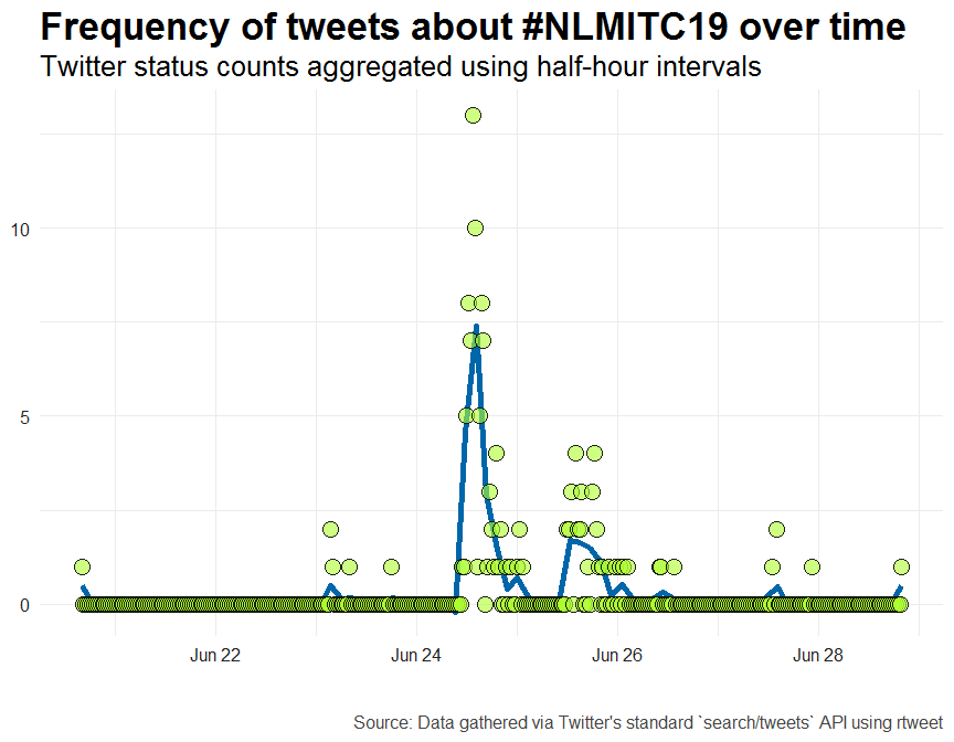
rt %>%
  ts_plot("30 minutes", color = "transparent") +
  geom_smooth(method = "loess",
              se = FALSE,
              span = 0.05,
              size = 2,
              color = "#0066aa") +
  geom_point(size = 5,
             shape = 21,
             fill = "#ADFF2F99",
             color = "#000000dd") +

  # ggplot2 theme
  theme_minimal(base_size = 15) +
  theme(axis.text = element_text(colour = "#222222"),
        plot.title = element_text(size = rel(1.7), face = "bold"),
        plot.subtitle = element_text(size = rel(1.3)),
        plot.caption = element_text(colour = "#444444")) +

  # Caption information
  labs(title = "Frequency of tweets about #NLMITC19 over time",
       subtitle = "Twitter status counts aggregated using half-hour intervals",
       caption = "\n\nSource: Data gathered via Twitter's standard `search/tweets` API using rtweet",
       x = NULL, y = NULL)
Makes sense considering there were two days of conference time.
rt %>%
  group_by(screen_name) %>%
  summarise(tweets = n()) %>%
  ggplot(aes(x = tweets, y = reorder(screen_name, tweets))) +
  geom_point() +

  # Theme styling information
  theme_minimal(base_size = 15) +
  theme(axis.text = element_text(colour = "#222222"),
        plot.title = element_text(size = rel(1.7), face = "bold"),
        plot.subtitle = element_text(size = rel(1.3)),
        plot.caption = element_text(colour = "#444444")) +

  # Labels
  labs(title = "Top tweeters using\n#NLMITC19 or #NLMIT19",
       x = "Total number of tweets",
       y = "Twitter username",
       caption = "\n\nSource: Data gathered via Twitter's standard `search/tweets` API using rtweet")
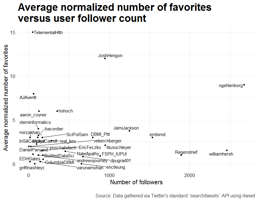
Do more followers have more popular tweets?
I take the average number of favorite of an individual’s tweets and normalize it based on the total number of tweets.
rt %>%
  # Preprocess and count average favorites normalized by number of tweets
  group_by(screen_name) %>%
  mutate(avg_fav = mean(favorite_count)) %>%
  mutate(avg_norm_fav = avg_fav / n()) %>%
  ungroup() %>%
  select(screen_name, avg_fav, avg_norm_fav, followers_count) %>%
  distinct() %>%

  # Offset to not create infinite values when log transforming
  mutate(followers_count = followers_count + 0.001) %>%
  mutate(avg_norm_fav = avg_norm_fav + 0.001) %>%

  # Plot results
  ggplot(aes(x = followers_count, y = avg_norm_fav, label = screen_name)) +
  geom_text_repel() +
  geom_point() +

  # Use log-scale for x-axis and y-axis
  labs(title = "Average normalized number of favorites\nversus user follower count",
       x = "Number of followers",
       y = "Average normalized number of favorites",
       caption = "\nSource: Data gathered via Twitter's standard `search/tweets` API using rtweet") +

  # Theme styling information
  theme_minimal(base_size = 15) +
  theme(axis.text = element_text(colour = "#222222"),
        plot.title = element_text(size = rel(1.7), face = "bold"),
        plot.subtitle = element_text(size = rel(1.3)),
        plot.caption = element_text(colour = "#444444"))
rt_no_stop <- rt %>%
  # Just look at tweet text
  select(text, favorite_count) %>%

  # Remove web links
  mutate(text = str_replace_all(text, "https?[:graph:]+", "'")) %>%

  # Remove mentions
  # Rule are that names are alphanumeric and can have underscores.
  # Names can also be preceeded with "." or end with some punctuation
  # Twitter:
  #   help.twitter.com/en/managing-your-account/twitter-username-rules
  # To avoid emails:
  #   stackoverflow.com/questions/4424179/how-to-validate-a-twitter-username-using-regex#comment21201837_4424288
  mutate(text = str_replace_all(text,
                                "\\.?@([:alnum:]|_){1,15}(?![.A-Za-z])[:graph:]?",
                                "")) %>%

  # Tokenize text to just single words
  unnest_tokens(word, text) %>%

  # Remove stop words (e.g., "a", "the", "and", etc)
  anti_join(get_stopwords())
## Joining, by = "word"


# Get average number of favorites
rt_word_avg_fav <- rt_no_stop %>%
  # Average favorite count
  group_by(word) %>%
  summarize(avg_fav = mean(favorite_count))


# Count number of mentions
rt_counts <- rt_no_stop %>%
  # Create word counts
  count(word, sort = TRUE)


# Filter low counts and join counts and average favorite score
chatter_rt <- rt_counts %>%
  filter(n > 1) %>%
  filter(word != "nlmitc19") %>%
  left_join(rt_word_avg_fav, by = "word")
Code below modified from “RIP wordclouds, long live CHATTERPLOTS”.
chatter_rt %>%
  # Add small offset average favorite counts because some are zero and we log
  # transform, which can introduce infinite values
  mutate(avg_fav = avg_fav + 0.001) %>%

  # Gather just top 100 mentions
  top_n(100, wt = n) %>%

  ggplot(aes(x = avg_fav, y = n, label = word)) +
  geom_text_repel(segment.alpha = 0,
                  aes(colour = avg_fav, size = n)) +

  # Set color gradient,log transform & customize legend
  scale_color_gradient(low = "green3", high = "violetred",
                       trans = "log10",
                       guide = guide_colourbar(direction = "horizontal",
                                               title.position = "top")) +
  # Set word size range & turn off legend
  scale_size_continuous(range = c(3, 10),
                        guide = FALSE) +

  # Use log-scale for x-axis
  scale_x_log10() +
  ggtitle(paste0("Top 100 words from ",
                  nrow(rt),
                 " #NLMITC19 tweets, by frequency"),
          subtitle = "Word frequency (size) ~ Avg number of favorites (color)") +
  labs(y = "Word frequency across all tweets",
       x = "Avg number of favorites in tweets containing word (log scale)",
       colour = "Avg num of favs (log)") +

  # minimal theme & customizations
  theme_minimal() +
  theme(legend.position = c(0.20, 0.99),
        legend.justification = c("right","top"),
        panel.grid.major = element_line(colour = "whitesmoke"))
sessionInfo()
## R version 3.5.0 (2018-04-23)
## Platform: x86_64-w64-mingw32/x64 (64-bit)
## Running under: Windows 7 x64 (build 7601) Service Pack 1
##
## Matrix products: default
##
## locale:
## [1] LC_COLLATE=English_United States.1252
## [2] LC_CTYPE=English_United States.1252
## [3] LC_MONETARY=English_United States.1252
## [4] LC_NUMERIC=C
## [5] LC_TIME=English_United States.1252
##
## attached base packages:
## [1] stats     graphics  grDevices utils     datasets  methods   base
##
## other attached packages:
##  [1] rtweet_0.6.8    ggrepel_0.8.0   tidytext_0.2.0  forcats_0.4.0
##  [5] stringr_1.4.0   dplyr_0.8.0.1   purrr_0.3.2     readr_1.3.1
##  [9] tidyr_0.8.3     tibble_2.1.1    ggplot2_3.1.0   tidyverse_1.2.1
##
## loaded via a namespace (and not attached):
##  [1] tidyselect_0.2.5  xfun_0.5          haven_2.1.0
##  [4] lattice_0.20-38   colorspace_1.4-1  generics_0.0.2
##  [7] htmltools_0.3.6   SnowballC_0.6.0   yaml_2.2.0
## [10] rlang_0.3.2       pillar_1.3.1      glue_1.3.1
## [13] withr_2.1.2       modelr_0.1.4      readxl_1.3.1
## [16] plyr_1.8.4        munsell_0.5.0     gtable_0.3.0
## [19] cellranger_1.1.0  rvest_0.3.2       evaluate_0.13
## [22] labeling_0.3      knitr_1.22        broom_0.5.1
## [25] tokenizers_0.2.1  Rcpp_1.0.1        scales_1.0.0
## [28] backports_1.1.3   jsonlite_1.6      stopwords_0.9.0
## [31] hms_0.4.2         digest_0.6.18     stringi_1.4.3
## [34] grid_3.5.0        cli_1.1.0         tools_3.5.0
## [37] magrittr_1.5      lazyeval_0.2.2    janeaustenr_0.1.5
## [40] crayon_1.3.4      pkgconfig_2.0.2   Matrix_1.2-16
## [43] xml2_1.2.0        lubridate_1.7.4   assertthat_0.2.1
## [46] rmarkdown_1.12    httr_1.4.0        rstudioapi_0.10
## [49] R6_2.4.0          nlme_3.1-137      compiler_3.5.0


