Regression Analysis in Statsmodels - Lab

Introduction

In the previous code along, we looked all the requirements for running an ols simple regression using statsmodels. We worked with a toy example to understand the process and all the necessary steps that must be performed. In this lab , we shall look at a slightly more complex example to study the impact of spendings in different advertising channels of total sales.

Objectives

You will be able to:

Set up an analytical question to be answered by regression analysis
Study regression assumptions for real world datasets
Visualize the results of regression analysis

Let's get started

In this lab, we will work with the "Advertising Dataset" which is a very popular dataset for studying simple regression. The dataset is available at Kaggle, but we have already downloaded for you. It is available as "Advertising.csv". We shall use this dataset to ask ourselves a simple analytical question:

The Question

Which advertising channel has a strong relationship with sales volume, and can be used to model and predict the sales.

Step 1: Read the dataset and inspect its columns and 5-point statistics

# Load necessary libraries and import the data

# Check the columns and first few rows

.dataframe tbody tr th {
    vertical-align: top;
}

.dataframe thead th {
    text-align: right;
}

</style>

	TV	radio	newspaper	sales
1	230.1	37.8	69.2	22.1
2	44.5	39.3	45.1	10.4
3	17.2	45.9	69.3	9.3
4	151.5	41.3	58.5	18.5
5	180.8	10.8	58.4	12.9

# Get the 5-point statistics for data

.dataframe tbody tr th {
    vertical-align: top;
}

.dataframe thead th {
    text-align: right;
}

</style>

	TV	radio	newspaper	sales
count	200.000000	200.000000	200.000000	200.000000
mean	147.042500	23.264000	30.554000	14.022500
std	85.854236	14.846809	21.778621	5.217457
min	0.700000	0.000000	0.300000	1.600000
25%	74.375000	9.975000	12.750000	10.375000
50%	149.750000	22.900000	25.750000	12.900000
75%	218.825000	36.525000	45.100000	17.400000
max	296.400000	49.600000	114.000000	27.000000

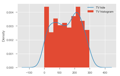
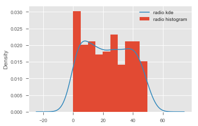
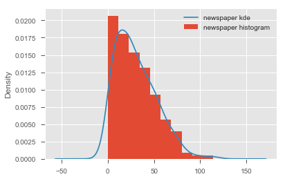
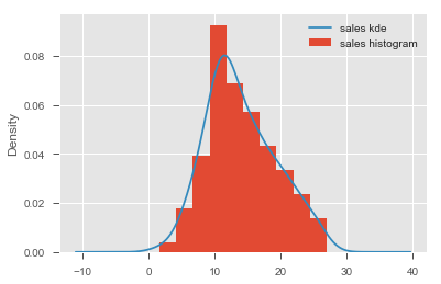
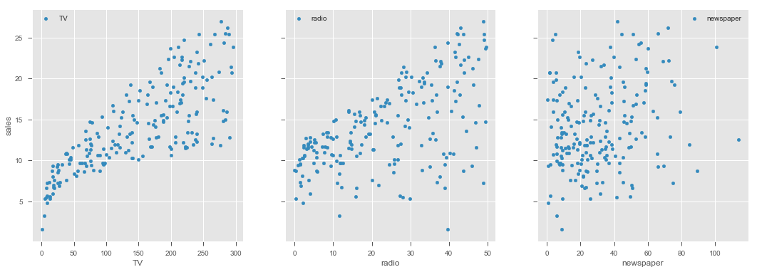
# Describe the contents of this dataset

Step 2: Plot histograms with kde overlay to check for the normality of the predictors

# For all the variables, check if they hold normality assumption

# Record your observations on normality here

Remember . Nothing is perfect . So be positive

Step 3: Test for the linearity assumption.

Use scatterplots to plot each predictor against the target variable

# visualize the relationship between the preditors and the target using scatterplots

# Record yor observations on linearity here

Conclusion so far !

Based on above initial checks, we can confidently say that TV and radio appear to be good predictors for our regression analysis. Newspaper is very heavily skewed and also doesnt show any clear linear relationship with the target.

We shall move ahead with our analysis using TV and radio , and count out the newspaper due to the fact that data violates ols assumptions

Note: Kurtosis can be dealt with using techniques like log normalization to "push" the peak towards the center of distribution. We shall talk about this in the next section.

Step 4: Run a simple regression in `statsmodels` with TV as a predictor

# import libraries

# build the formula 

# create a fitted model in one line

Step 5: Get regression diagnostics summary

OLS Regression Results

Dep. Variable:	sales	R-squared:	0.612
Model:	OLS	Adj. R-squared:	0.610
Method:	Least Squares	F-statistic:	312.1
Date:	Fri, 12 Oct 2018	Prob (F-statistic):	1.47e-42
Time:	21:04:59	Log-Likelihood:	-519.05
No. Observations:	200	AIC:	1042.
Df Residuals:	198	BIC:	1049.
Df Model:	1
Covariance Type:	nonrobust

	coef	std err	t	P>\|t\|	[0.025	0.975]
Intercept	7.0326	0.458	15.360	0.000	6.130	7.935
TV	0.0475	0.003	17.668	0.000	0.042	0.053

Omnibus:	0.531	Durbin-Watson:	1.935
Prob(Omnibus):	0.767	Jarque-Bera (JB):	0.669
Skew:	-0.089	Prob(JB):	0.716
Kurtosis:	2.779	Cond. No.	338.

Record your observations on "Goodness of fit"

Note here that the coefficients represent associations, not causations

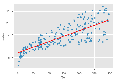
Step 6: Draw a prediction line with data points omn a scatter plot for X (TV) and Y (Sales)

Hint: We can use model.predict() functions to predict the start and end point of of regression line for the minimum and maximum values in the 'TV' variable.

# create a DataFrame with the minimum and maximum values of TV

# make predictions for those x values and store them


# first, plot the observed data and the least squares line

      TV
0    0.7
1  296.4
0     7.065869
1    21.122454
dtype: float64

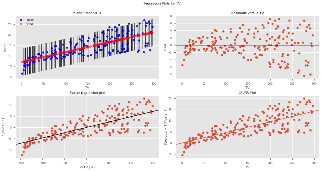
Step 7: Visualize the error term for variance and heteroscedasticity

# Record Your observations on residuals

Next, repeat above for radio and go through the same process, recording your observations

R-Squared: 0.33203245544529525
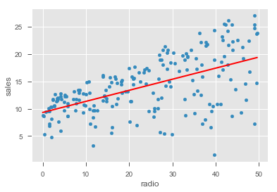
Intercept    9.311638
radio        0.202496
dtype: float64

model.summary()

OLS Regression Results

Dep. Variable:	sales	R-squared:	0.332
Model:	OLS	Adj. R-squared:	0.329
Method:	Least Squares	F-statistic:	98.42
Date:	Fri, 12 Oct 2018	Prob (F-statistic):	4.35e-19
Time:	20:52:55	Log-Likelihood:	-573.34
No. Observations:	200	AIC:	1151.
Df Residuals:	198	BIC:	1157.
Df Model:	1
Covariance Type:	nonrobust

	coef	std err	t	P>\|t\|	[0.025	0.975]
Intercept	9.3116	0.563	16.542	0.000	8.202	10.422
radio	0.2025	0.020	9.921	0.000	0.162	0.243

Omnibus:	19.358	Durbin-Watson:	1.946
Prob(Omnibus):	0.000	Jarque-Bera (JB):	21.910
Skew:	-0.764	Prob(JB):	1.75e-05
Kurtosis:	3.544	Cond. No.	51.4

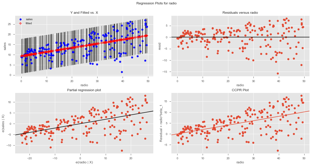
# Record your observations here for goodnes of fit

The Answer

Based on above analysis, we can conclude that none of the two chosen predictors is ideal for modeling a relationship with the sales volumes. Newspaper clearly violated normality and linearity assumptions. TV and radio did not provide a high value for co-efficient of determination - TV performed slightly better than the radio. There is obvious heteroscdasticity in the residuals for both variables.

We can either look for further data, perform extra pre-processing or use more advanced techniques.

Remember there are lot of technqiues we can employ to FIX this data.

Whether we should call TV the "best predictor" or label all of them "equally useless", is a domain specific question and a marketing manager would have a better opinion on how to move forward with this situation.

In the following lesson, we shall look at the more details on interpreting the regression diagnostics and confidence in the model.

Summary

In this lesson, we ran a complete regression analysis with a simple dataset. We looked for the regression assumptions pre and post the analysis phase. We also created some visualizations to develop a confidence on the model and check for its goodness of fit.

evanavaughan/dsc-01-10-13-regression-statsmodels-lab-nyc-career-ds-102218