In this course we cover the following topics:
- Week 1
- Introduction
- Linear Regression with One Variable
- Linear Algebra Review
- Week 2
- Linear Regression with Multiple Variables
- Octave/Matlab Tutorial
- Week 3
- Logistic Regression
- Regularization
- Week 4
- Neural Networks: Representation
- Week 5
- Neural Networks: Learning
- Week 6
- Advice for Applying Machine Learning
- Machine Learning System Design
- Week 7
- Support Vector Machines
- Week 8
- Unsupervised Learning
- Dimensionality Reduction
- Week 9
- Anomaly Detection
- Recommender Systems
- Week 10
- Large Scale Machine Learning
- Week 11
- Photo Optical Character Recognition
Notes from each section will be appended here as well as available to view in each subfolder for each week.
In Week 1 we cover the following topics:
- Linear Regression with One Variable
- Linear Algebra (Review)
Machine Learning
- Grew out of work in AI
- New capability for computers
Examples:
- Database mining: Large datasets from growth of automation/web. E.g., Web click data, medical records, biology, engineering
- Applications can’t program by hand: E.g., Autonomous helicopter, handwriting recognition, most of Natural Language Processing (NLP), Computer Vision
- Self-customizing programs: E.g., Amazon, Netflix product recommendations
What is machine learning?
-
Arthur Samuel (1959). Machine Learning: "Field of study that gives computers the ability to learn without being explicitly programmed."
-
Tom Mitchell (1998) Well-posed Learning Problem: "A computer program is said to learn from experience E with respect to some task T and some performance measure P, if its performance on T, as measured by P, improves with experience E."
Two main types of machine learning algorithms:
-
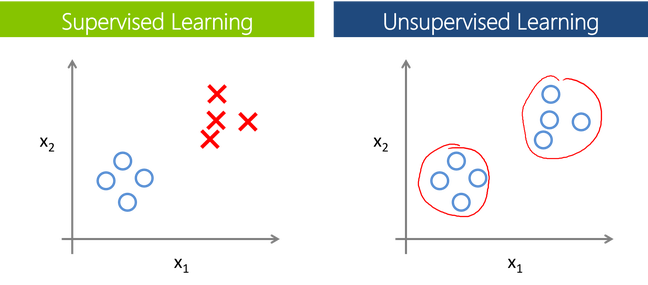
Supervised learning: The majority of practical machine learning problems. We know the correct answers, the algorithm iteratively makes predictions on the training data and is corrected. Learning stops when the algorithm achieves an acceptable level of performance. We can group supervised learning problems into:
- Regression problems: When the output variable is a real value e.g., "dollars" or "weight".
- Classification problems: When the output variable is a category e.g., "black" or "white".
-
Unsupervised learning: When there exists input data and no corresponding output variables. The goal for unsupervised learning is to model the underlying structure or distribution in the data in order to learn more about the data. We can group unsupervised learning problems into:
- Clustering problems: When we want to discover the inherent groupings in the data e.g., grouping customers by purchasing behavior.
- Association problems: When we want to discover rules that describe large portions of our data e.g., people that buy X also tend to buy Y.
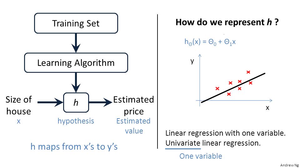
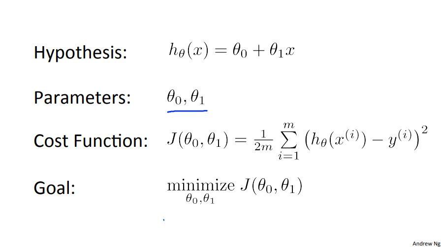
In a linear regression problem we predict a real-valued output using existing data that is the "right answer" for each example in the data. Furthermore, we can represent the data with a hypothesis function and use a cost function (squared error function) to minimize the parameters of the hypothesis.
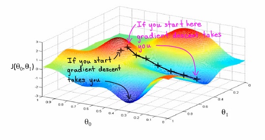
A way of minimizing the cost function is to use the gradient descent method. Gradient descent is an optimization algorithm used to find the values of parameters (coefficients) of a function (f) that minimizes a cost function (cost).
Matrices and vectors
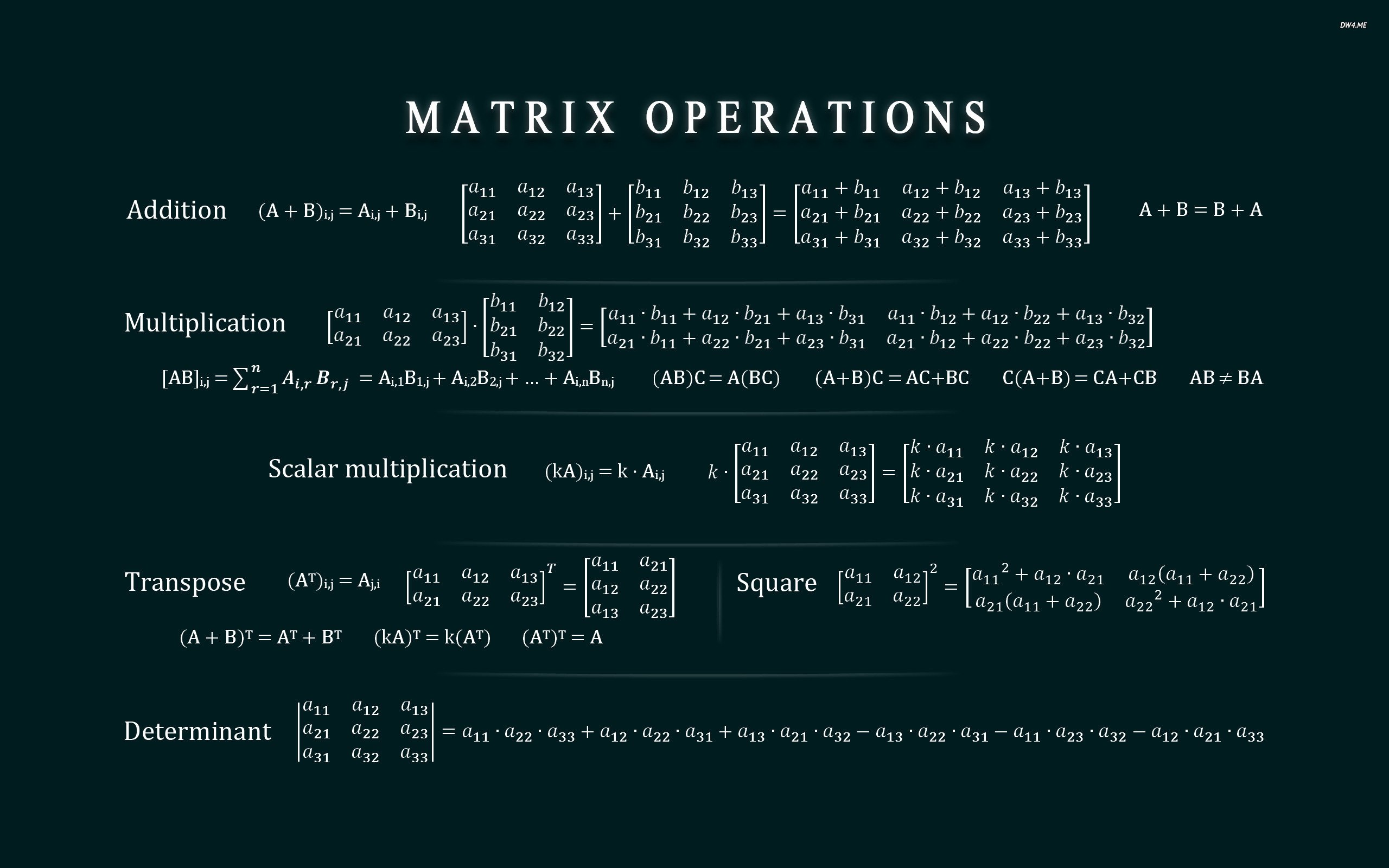
- Dimensions of matrix: rows x columns
In Week 2 we cover the following topics:
- Linear Regression with Multiple Variables
- Octave/Matlab Tutorial
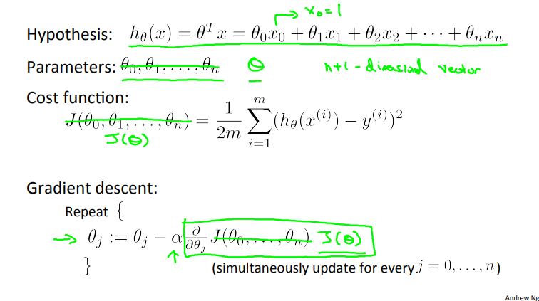
Linear regression with multiple variables is not too different than linear regression for single variables. When dealing with multiple variables, we must change the hypothesis, cost function, and gradient descent algorithm to represent multiple features. One way to do this is by using vector notation. An example of linear regression with multiple variables setup is denoted in Figure 2-1.
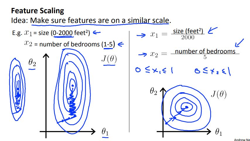
Feature scaling: make sure features are on a similar scale. One technique used to accomplish this is by using mean normalization. Feature scaling could drastically change the appearance of a graph and therefore, drastically improve the precision accuracy of a model (see Figure 2-2 for impacts of feature scaling).
Learning rate: Specified step-size the algorithm (in this case the gradient descent algorithm) takes at each iteration when trying to minimize the cost function.
In general, if the learning rate:
- Is too small, the convergence could be expected to happen slower than normal
- Is too large, the cost function may not decrease on every iteration and may not converge
Other regression techniques:
- Polynomial regression: Differs from linear regression with the addition of an nth degree term.
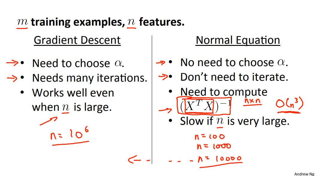
- Normal equation: Method to solve for the function parameters (commonly denoted by theta) analytically.
In Week 3 we cover the following topics:
- Logistic Regression
- Regularization
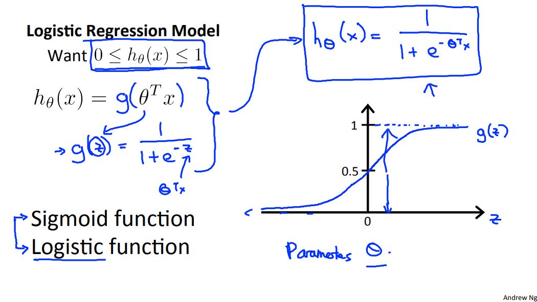
Logistic regression is intended for binary (two-class) classification problems. It will predict the probability of an instance belonging to the default class, which can be snapped into a 0 or 1 classification.
A logistic regression model could be represented as follows:
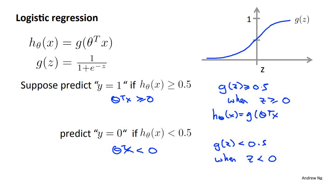
We can use a decision boundary to make predictions:
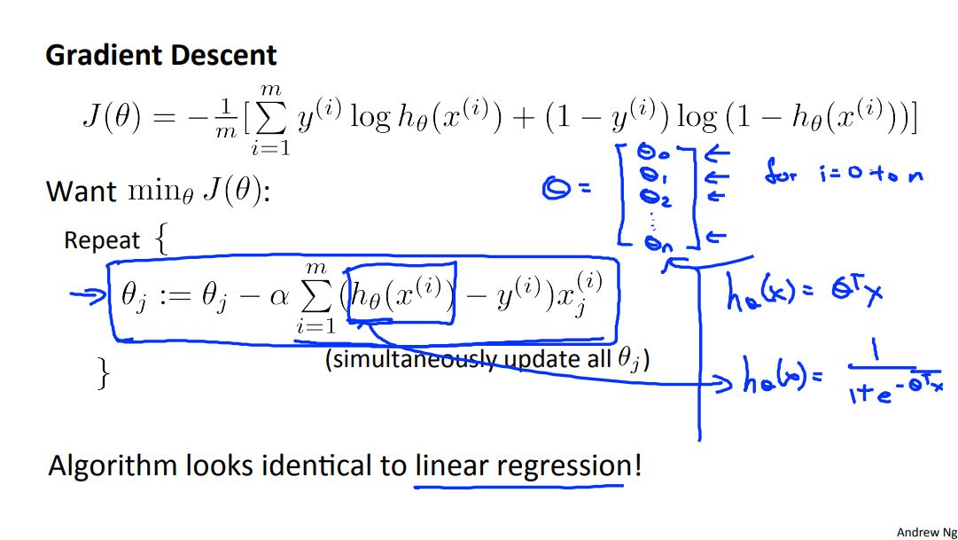
Additionally, the cost function and gradient descent algorithm for logistic regression looks fairly similar to that of linear regression:
In addition to linear and logistic regression techniques, we can also use optimization algorithms such as conjugate gradient, BFGS, L-BFGS, etc. The advantages of using optimization algorithms is that we do not manually have to pick the step-size variable. Optimization algorithms tend to be faster than gradient descent.
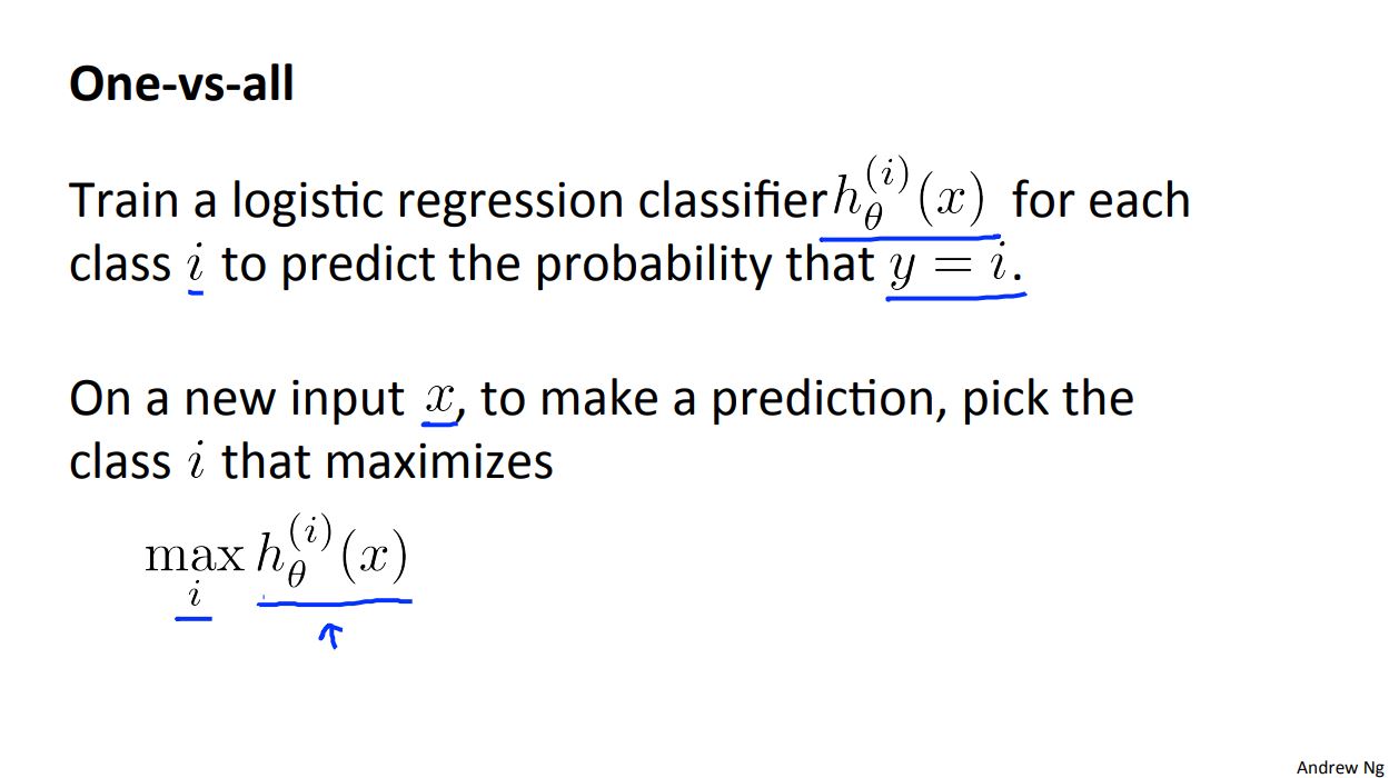
Multi-class classification: When there is more than one class, we can apply the one-vs-all method:
Overfitting: If we have too many features, the learned hypothesis may fit the training set very well, but fail to generalize to new examples (predict prices on new examples).
To address overfitting we can do the following:
- Reduce the number of features
- Manually select which features to keep
- Model selection algorithm
- Regularization
- Keep all the features, but reduce magnitude/values of parameters
- Works well when we have a lot of features, each of which contributes a bit to predicting the output.
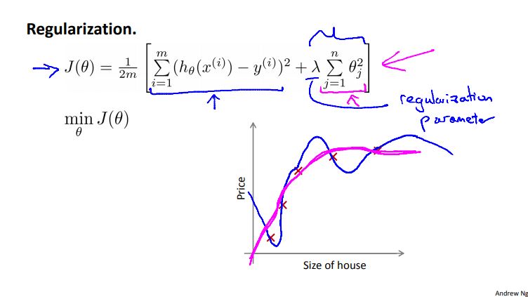
The cost function for regularization incudes an extra parameter to the cost function:
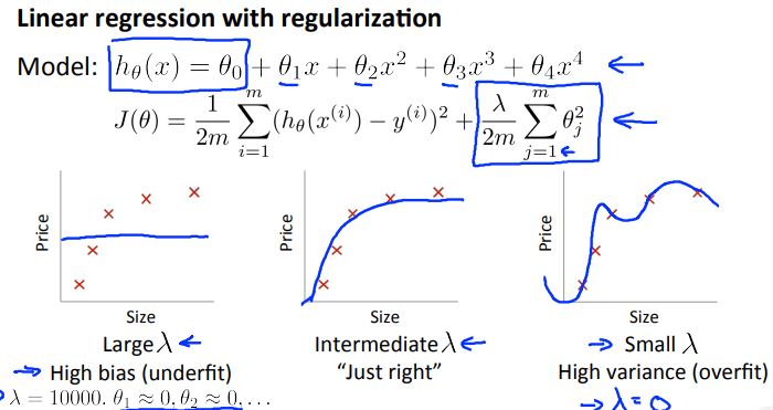
We do not want the lambda setting to be too small or else it will result in overfitting. Conversely, we do not want the lambda setting to be too large or else minimization of the cost function will result in underfitting.
The regularization parameter can be added to a linear or a logistic cost function as well as a gradient descent.
In Week 4 we cover the following topics:
- Neural Networks: Representation
Neural networks originated from algorithms that try to mimic the brain. The use of such algorithms became popular in the 80s and early 90s but soon diminished in the late 90s. Today, neural networks are being used for many applications.
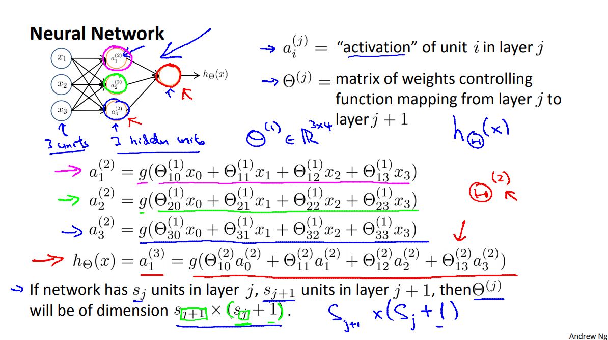
A neural network could be represented as follows:
Where the activation terms denoted by "a" occur in layer 2 to layer n (hidden layer). Alternatively, neural networks can be vectorized.
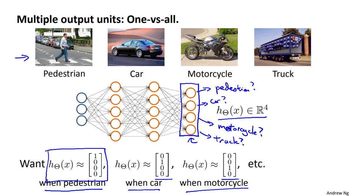
When trying to classify more than one output units a representation model could look like this:
In Week 5 we cover the following topics:
- Neural Networks: Learning
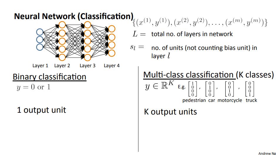
A neural network classification problem could be represented as either a binary or multi-class classification:
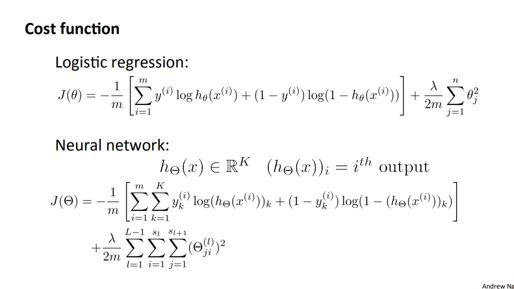
The cost function for a neural network could be represented as:
Which turns out to be quite similar to the logistic regression cost function.
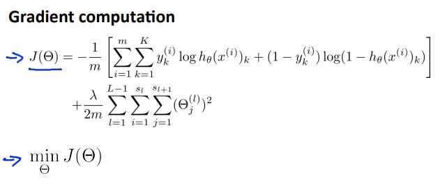
The gradient computation takes in the same idea as before: we seek to minimize the cost function. Figure 5-3 depicts the general equation needed to compute the gradient descent of a neural network and minimize the cost function:
Backpropagation is at the core of how neural networks learn.
To include backpropagation we would first need to have our neural network defined and an error function. In backpropagation, the final weights are calculated first and the first weights are calculated last. This allows for the efficient computation of the gradient at each layer.
In general, we forward propagate to get the output and compare it with the real value to get the error. Then, we backpropagate to minimize the error (find the derivative of error with respect to each weight then subtract this value from the weight value). This process repeats and continues until we reach a minima for error value.
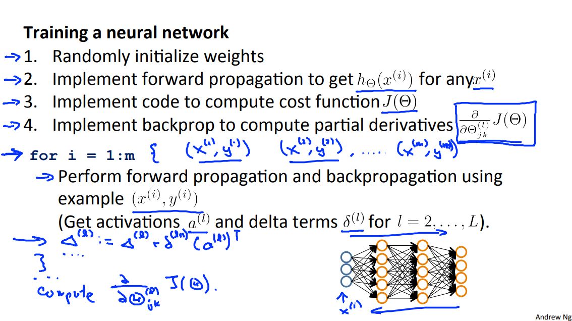
To summarize on how to train a neural network:
In addition to the steps proposed in Figure 5-4:
- Use gradient checking to compare the partial derivative of the cost function with respect to the weights computed using backpropagation versus using numerical estimate of gradient of the cost function
- Disable the gradient checking code
- Use gradient descent or advanced optimization method with backpropagation to try to minimize the cost function as a function of the weights
In Week 6 we cover the following topics:
- Advice for Applying Machine Learning
When deciding on what to try next during machine learning algorithm development, there are steps that should be considered.
An example could be if we implemented regularized linear regression to predict housing prices but the hypothesis makes unacceptable large errors in its predictions. In this case we should try to:
- Get more training examples
- Get additional features
A diagnostic is a test you can run to gain insight what is/isn't working with a learning algorithm, and gain guidance as to how best to improve its performance. Although diagnostics can take time to implement, doing so can be a very good use of time.
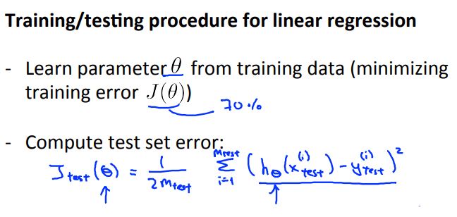
The training/testing procedure for linear regression is depicted in Figure 6-1.
Likewise, the training/testing procedure for logistic regression is as follows:
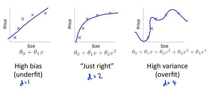
What does it mean when we say our model has bias or variance?
- Bias -> underfit
- Variance -> overfit
Figure 6-3 depicts an example of bias and variance
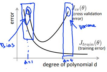
There are two types of errors we care about when dealing with bias and variance:
- Training error
- Cross validation error
The training error can be represented as a function whose error decreases with additional polynomial terms. In contrast, the cross validation error can be represented as a parabolic function where there is a specific degree of polynomial terms that would yield a minimum error.
In general, when the learning algorithm has bias:
- Training error will be high
- Cross validation error will be approximately the same as the training error
When the learning algorithm has variance:
- Training error will be low
- The cross validation error will be much greater than the training error
Linear regression with regularization also has bias or variance depending on the value of lambda.
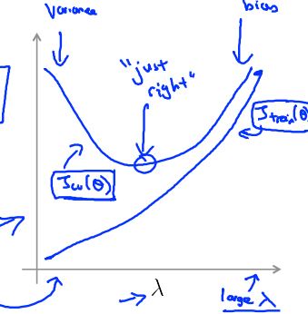
Similar to the training error and cross validation error for non-regularized algorithms, regularized algorithms have a parabolic cross validation where a specific value of lambda minimizes the bias/variance. However, the bias increases as the lambda value is increased for the training error.
If a learning algorithm is suffering from high bias, getting more training data will not (by itself) help much. However, if a learning algorithm is suffering from high variance, getting more training data is likely to help.
Revisiting the "next steps" to debugging an algorithm:
- Getting more training examples -> Fixes high variance
- Try smaller sets of features -> Fixes high variance
- Try getting additional features -> Fixes high bias
- Try adding polynomial features -> Fixes high bias
- Try decreasing lambda -> Fixes high bias
- Try increasing lambda -> Fixes high bias
When it comes to neural networks:
- Smaller neural networks have fewer parameters and are more prone to underfitting but are computationally cheaper
- Larger neural networks have more parameters and are more prone to overfitting (computationally more expensive)
We typically use regularization to address overfitting for neural networks.
Suppose we build a spam classifier where x = features of email and y = spam or not spam (1 or 0). In practice, we would take the most frequently occurring n words (10,000 to 50,000) in training set, rather than manually pick 100 words.
What is the best use of time to make it have low error?
- Start with a simple algorithm that you can implement quickly then implement it and test on cross validation data
- Plot learning curves to decide if more data, more features, etc. are likely to help
- Error analysis: manually examine the examples (cross validation set) that your algorithm made errors on then see if you spot any systematic trend in what type of example it is making errors on
For error metrics, we can use a cancer classification example where we have 1% error on test set where only 0.5% of patients have cancer. In this case we introduce precision and recall:
- Precision: Of all patients where we predicted y = 1, what fraction actually has cancer?
- Recall: Of all patients that actually have cancer, what fraction did we correctly detect as having cancer?
There is a trade-off between precision and recall:
- If we wanted to predict y = 1 only when very confident we would have higher precision and lower recall.
- If we wanted to avoid missing too many cases of cancer we would have higher recall and lower precision
- In general we want to predict 1 if the hypothesis output is greater than the threshold
When designing a high accuracy learning system, we want to:
- Have as much data as possible
- Use a learning algorithm with many parameters (e.g. logistic regression/linear regression with many features; neural network with many hidden units)
The cost of training will be small for low bias algorithms and using a very large training set will result in low variance.
In Week 7 we cover the following topics:
- Support Vector Machines
Support vector machines (SVMs) are supervised learning models with associated learning algorithms that analyze data used for classification and regression analysis.
Given a set of training examples, each marked as belonging to one or the other of two categories, an SVM training algorithm builds a model that assigns new examples to one category or the other, making it a non-probabilistic binary linear classifier.
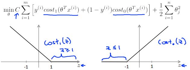
We can start by exploring an alternate logistic regression algorithm depicted in Figure 7-1.
In comparison, the SVM hypothesis can be written as follows:
If we look within the brackets of the equation depicted in Figure 7-2, we can extract information on the SVM decision boundary:
- When y(i) = 1, we want the term within the cost function to be greater than or equal to 1
- When y(i) = 0, we want the term within the cost function to be less than or equal to -1
We can use a SVM as a large margin classifier. In large margin classification, a perceptron is a hyperplane that separates classes (see previous link on large margin classifiers for more details).
In machine learning, kernel methods are a class of algorithms for pattern analysis, whose best known member is the SVM. The general task of pattern analysis is to find and study general types of relations (e.g. clusters, rankings, principal components, correlations, classifications) in datasets.
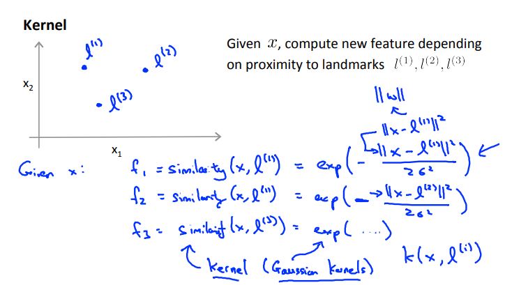
Similarity kernels works as follows:
- If the given data x is close to the landmarks, then the similarity f will be approximately equal to 1
- If the given data x is far from the landmarks, then the similarity f will be approximately equal to 0
To use kernels with SVMs simply refer to Figure 7-2 and replace the x(i) terms with f(i) similarity term.
SVM parameters are chosen based on the following factors:
In practice, we follow several steps to implement SVM in our projects:
- Use SVM software package (e.g. liblinear, libsvm, ...) to solve for the theta parameters
- Specify choice of parameter C and choice of kernel (similarity function):
- No kernel (linear kernel), where we predict y = 1 if the hypothesis (the term in the cost function in Figure 7-2) is greater than or equal to zero
- Gaussian kernel (Figure 7-4), where l(i) = x(i)
We must note that for a Gaussian kernel, we should perform feature scaling before using the Gaussian kernel, otherwise our model will not perform as intended. Additionally, not all similarity functions make valid kernels. We need to satisfy a technical condition called Mercer's Theorem to make sure SVM packages do not diverge and run as intended.
The table below address the differences between logistic regression vs SVMs:
- n = number of features
- m = number of training examples
- For the case where n is small and m is large, it is recommended to create/add more features first then use logistic regress or SVM without a kernel
| Case | Logistic regression | SVMs |
|---|---|---|
| n is large | Ok to use | Use linear kernel (SVM without a kernel) |
| n is small/m is intermediate | Not preferred | Use SVM with Gaussian kernel |
| n is small/m is large | Ok to use | Use linear kernel (SVM without a kernel) |
Additionally, applying neural networks to these problems will most likely work well but may be slower to train.
In Week 8 we cover the following topics:
- Unsupervised Learning
- Dimensionality Reduction
Unsupervised learning is a machine learning technique for finding hidden patterns or intrinsic structures in data. In other words, unsupervised learning is used to draw inferences from datasets consisting of input data without labeled responses.
The most common unsupervised learning method is cluster analysis, which is used for exploratory data analysis to find hidden patterns or grouping in data. The clusters are modeled using a measure of similarity which is defined upon metrics such as Euclidean or probabilistic distance.
Some applications of clustering include:
- Market segmentation
- Social network analysis
- Organize computing clusters
- Astronomical data analysis
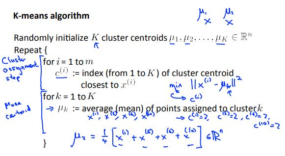
The K-means algorithm is one of the algorithms used for clustering. K is the number of clusters and the training set can me any number from 1 to m training sets. The steps to the K-means algorithm is highlighted in Figure 8-1.
What the algorithm does in Figure 8-1 is effectively partitioning data into k distinct clusters based on distance to the centroid of a cluster. For an animation of how the K-means algorithm works with each iteration see this page for the standard K-means clustering algorithm
The K-means algorithm generally uses the random partition method to initialize the algorithm. This means that a cluster is randomly assigned to each observation and then proceeds to update step and compute the initial mean to be the centroid of the cluster's randomly assigned points.
There are many ways to choose the value of K, here are a couple:
- Elbow method - looking for the "drop" in the cost function as the K (number of clusters) increases.
- Downstream method - evaluating K-means based on a metric for how well it performs for that later purpose.
Dimensionality reduction is in the process of reducing the number of random variables under consideration by obtaining a set of principal variables. Dimensionality reduction can be divided into feature selection and feature extraction.
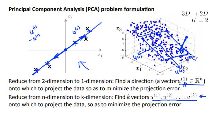
The main linear technique for dimensionality reduction is principal component analysis (PCA). PCA performs a linear mapping of the data to a lower-dimension space in such a way that the variance of the data in the low-dimensional representation is maximized.
Why should we use PCA?
- Compression:
- Reduce memory/disk needed to store data
- Speed up learning algorithm
- Visualization of data
When should we use PCA?
- We should use PCA if the raw data x(i) does not do what is intended, then implement PCA and consider using z(i) which is the mapped dataset.
However, what we don't want to do is end up using z(i) to reduce the number of features to k < n to prevent overfitting. Overfitting should be addressed by using regularization.
The recommended approach is to design the ML system first and run the program without using PCA.
In Week 9 we cover the following topics:
- Anomaly Detection
- Recommender Systems
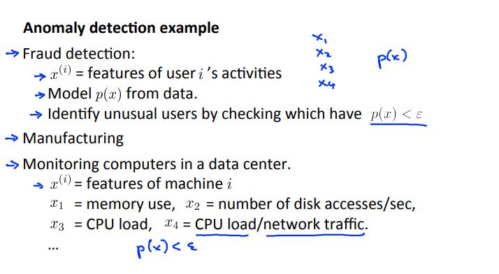
Anomaly detection is a technique used to identify unusual patterns that do not conform to expected behavior, called outliers. It has many applications in business, from intrusion detection (identifying strange patterns in network traffic that could signal a hack) to system health monitoring (spotting a malignant tumor in an MRI scan), and from fraud detection in credit card transactions to fault detection in operating environments.
Anomalies can be classified as:
-
Point anomalies: A single instance of data is anomalous if it's too far off from the rest. Business use case: Detecting credit card fraud based on "amount spent."
-
Contextual anomalies: The abnormality is context specific. This type of anomaly is common in time-series data. Business use case: Spending $100 on food every day during the holiday season is normal, but may be odd otherwise.
-
Collective anomalies: A set of data instances collectively helps in detecting anomalies. Business use case: Someone is trying to copy data form a remote machine to a local host unexpectedly, an anomaly that would be flagged as a potential cyber attack.
Figure 9-1 depicts an example of how anomaly detection could be setup.
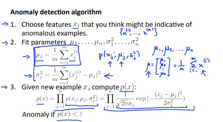
We can use Gaussian distribution to find any outliers in our data. Additionally, we can also use density estimation (the construction of an estimate based on observed data of an unobservable underlying probability density function) to build our anomaly detection algorithm as shown in Figure 9-2.
When developing a learning algorithm, making decisions is much easier if we have a way of evaluating our learning algorithm.
We can first fit our model to our training set and then on a cross validation test we can evaluate metrics such as:
- True positive, false positive, false, negative, true negative
- Precision/recall
- F-score
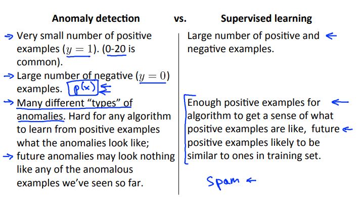
The differences between anomaly detection (recall that anomaly detection is an unsupervised learning technique) and supervised learning is shown in Figure 9-3.
In general, when conduction error analysis on anomaly detection we generally want our predictions to be large for normal examples and small for anomalous examples.
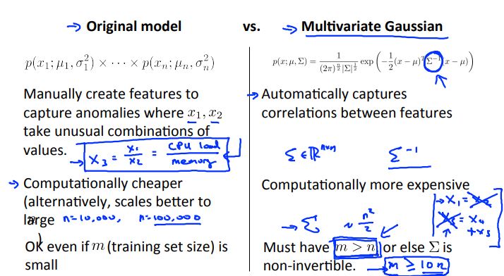
We can also compare the original model for anomaly detection against a multivariate Gaussian distribution model in Figure 9-4.
A recommender system is a subclass of information filtering system that seeks to predict the "rating" or "preference" a user would give to an item.
Recommender systems have become increasingly popular recent years, and are utilized in a variety of areas including movies, music, news, books, research articles, search queries, social tags, and products in general.
Recommender systems typically produce a list of recommendations in one of two ways – through collaborative filtering or through content-based filtering (also known as the personality-based approach):
- Collaborative filtering: approaches build a model from a user's past behavior (items previously purchased or selected and/or numerical ratings given to those items) as well as similar decisions made by other users. This model is then used to predict items (or ratings for items) that the user may have an interest in.
- Content-based filtering: approaches utilize a series of discrete characteristics of an item in order to recommend additional items with similar properties.
Figure 9-5 shows what the algorithm could look like for a content-based recommendation.
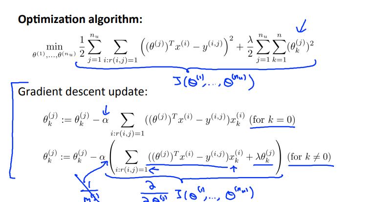
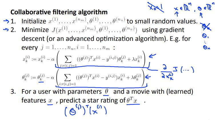
Collaborative filtering works differently by minimizing the training set data (x) and the parameters (theta) simultaneously. Figure 9-6 shows how one could setup the algorithm for such a problem.
Recommender systems can also be implemented in vectorized notation as well using techniques such as low rank matrix factorization and mean normalization
In Week 10 we cover the following topics:
- Large Scale Machine Learning
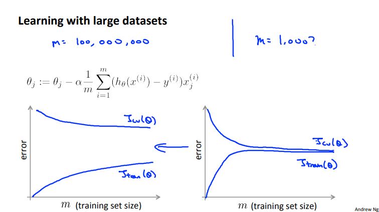
Often, it has been said in machine learning that: It's not who has the best algorithm that wins. It's who has the most data.
Below is a figure which depicts improvements made to our model based on a large dataset
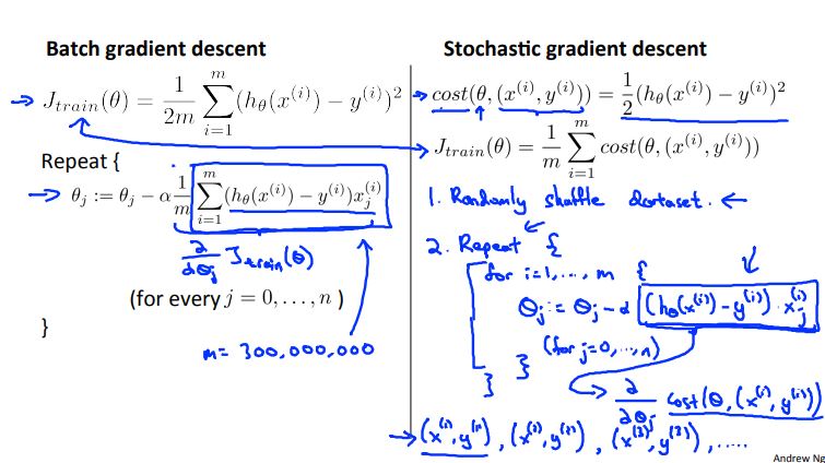
Stochastic gradient descent (SGD), also known as incremental gradient descent, is an iterative method for optimizing a differentiable objective function, a stochastic approximation of gradient descent optimization.
When the training set is enorm0ous and no simple formulas exist, evaluating the sums of gradients becomes very expensive, because evaluating the gradient requires evaluating all the summand functions' gradients. To economize on the computational cost at every iteration, stochastic gradient descent samples a subset of summand functions at every step. This is very effective in the case of large-scale machine learning problems.
Here are some things to note about SGD:
- In SGD, before for-looping, you need to randomly shuffle the training examples.
- In SGD, because it’s using only one example at a time, its path to the minima is noisier (more random) than that of the batch gradient. But it’s ok as we are indifferent to the path, as long as it gives us the minimum AND the shorter training time.
- Mini-batch gradient descent uses n data points (instead of 1 sample in SGD) at each iteration.
Figure 10-2 shows an example showing the set-up of both a batch gradient descent and SGD.
- Batch gradient descent: Use all m examples in each iteration.
- Stochastic gradient descent: Use 1 example in each iteration.
- Mini-batch gradient descent: Use b examples in each iteration.
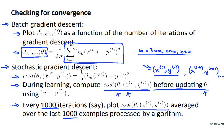
Like previous algorithms we need to check for convergence. Figure 10-3 depicts how we would do that for batch gradient descent and SGD.
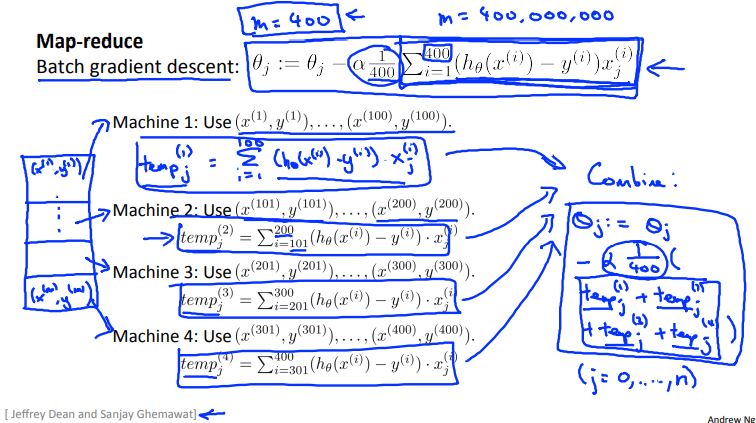
Some machine learning algorithms are too big to run on just one machine. We can solve this limitation by using the map-reduce technique.
Figure 10-4 shows how we might implement map-reduce for a batch gradient descent problem.
After each temp variables have been calculated, a "master server" will combine results of all temp variables to produce the final result.
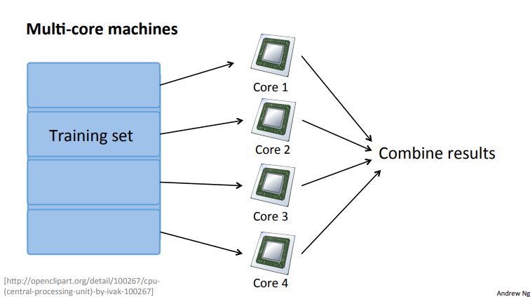
Many learning algorithms can be expressed as computing sums of functions over the training set.
Figure 10-5 shows an example of what map-reduce would look like on a multi-core machine.
In Week 11 we cover the following topics:
- Photo OCR
Below is the wiki definition of optical character recognition:
Optical character recognition (also optical character reader, OCR) is the mechanical or electronic conversion of images of typed, handwritten or printed text into machine-encoded text, whether from a scanned document, a photo of a document, a scene-photo (for example the text on signs and billboards in a landscape photo) or from subtitle text superimposed on an image (for example from a television broadcast).
Widely used as a form of information entry from printed paper data records — whether passport documents, invoices, bank statements, computerized receipts, business cards, mail, printouts of static-data, or any suitable documentation — it is a common method of digitizing printed texts so that they can be electronically edited, searched, stored more compactly, displayed on-line, and used in machine processes such as cognitive computing, machine translation, (extracted) text-to-speech, key data and text mining. OCR is a field of research in pattern recognition, artificial intelligence and computer vision.
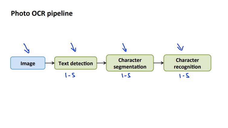
Figure 11-1 depicts the photo OCR pipeline - steps the computer takes to recognize characters - for a typical photo OCR problem.
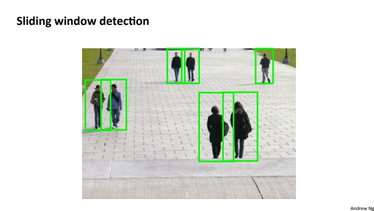
A sliding windows classifier utilizes aspect ratios (height to width ratios) of certain objects in images to determine whether or not a certain object in a particular image is of interest.
A large training set of positive and negative examples is required in order for the sliding windows technique to work.
Step size (typically 1 pixel) is specified for the algorithm of choice and the algorithm will run through the image 1 pixel at a time to try and detect the object of interest.
Resizing the aspect ratio of the box which is used to detect objects is often a step that happens in order to find objects at different locations in the image. Figure 11-2 depicts the results of using aspect ratios and resizing to detect pedestrians.
After text has been detected character segmentation determines whether or not a line can run through a particular image patch. A supervised learning algorithm can then be applied to classify what character is in an image patch.
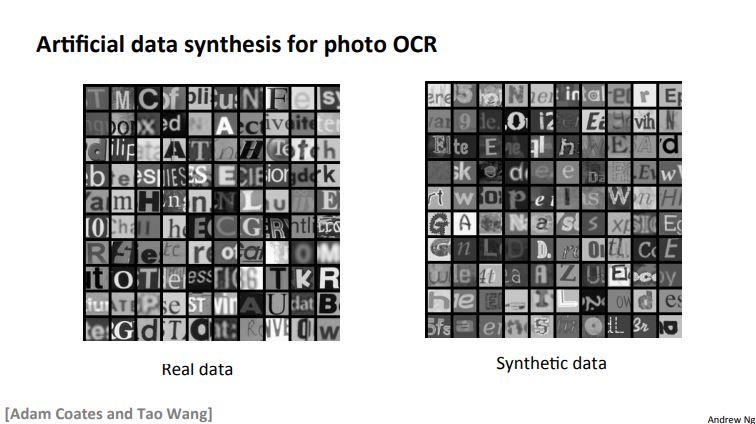
Synthesizing data allows the computer to determine the character even if it may look somewhat different (see Figure 11-3).
We can synthesize data by introducing distortions to our training set. However, we do have to be mindful when getting more data:
- Make sure we have low bias classifier before expending the effort (plot learning curves). We can increase the number of features/number of hidden units in our neural network until we have a low bias classifier.
- We have to ask ourselves "How much work would it be to get ten times as much data as we currently have?"
We have to keep in mind the errors due to each component (ceiling analysis) when working on our solution. By determining the error due to each component we can focus on areas which may require more work than others (improving component x might only yield 1% more accuracy but improving component y might yield 10% more accuracy).
