Selective, Interpretable and Motion Consistent Privacy Attribute Obfuscation for Action Recognition
CVPR 2024
Filip Ilic, He Zhao, Thomas Pock, Richard P. Wildes

The goal is to hide privacy relevant attributes without action recognition performance dropping. We show that it is not necessary to train action recognition and privacy networks in an adversarial fashion for effective obfuscation of privacy attributes while maintaining strong action recognition performance. We show that a system based on local privacy templates, deep features that capture template semantics and selective noise obfuscation that is animated with source video motion can uphold privacy without hindering action recognition. Our approach is unique compared to alternative recent approaches in terms of interpretability.

Environment Setup

git clone git@github.com:f-ilic/SelectivePrivacyPreservation.git
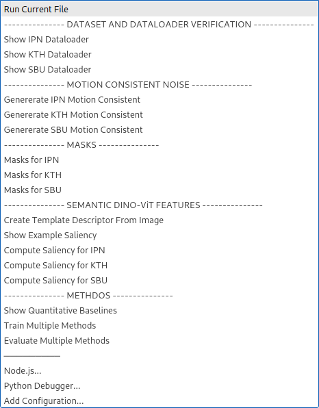
conda env create -f environment.yaml

Quickstart

We provide a launch.json for VSCode with all relevant run targets. Everything should work out of the box, after you set up the Datasets.

VSCode Run Targets

Otherwise

In case you are not running this from a IDE that sets the PYTHONPATH to the to the root directory (cwd) you need to manually set it with

export PYTHONPATH="/path/to/this/project:$PYTHONPATH"

Alternatively cd into the SelectivePrivacyPreservation/ and export PYTHONPATH="./" while exploring the codebase.

Datasets

Our evaluations utilize three datasets: IPN, SBU, KTH

Please download, extract, and organize each dataset in its original structure under data/<ipn|kth|sbu>. The directories should contain individual frames. For the IPN dataset, you'll need to download frames/frames[00-05].tar.gz. The KTH and SBU datasets are already organized as individual frames.

The dataset splits are provided in data/splits/<ipn|kth|sbu>.

Other intermediate results, such as saliency maps for each template, will be saved in data/ following the naming scheme <ipn|kth|sbu>_<modality>, where modality includes <masks|flow|afd>. Instructions for generating these modalities are provided below.

Use the sim postfix for similarity maps generated by the Matcher (<ipn|kth|sbu>_<template>_sim), and store them in data/. The dataloaders depend on this structure; modifications to source files will be necessary otherwise.

Dataset and Dataloader Verification

To verify correct dataset placement and functionality of the Anaconda environment, run:

python dataset/db_factory.py --datasetname ipn

Select the dataset with:

--datasetname DATASETNAME       options: [ 'ipn' | 'kth' | 'sbu' ]

This command launches a Matplotlib window, allowing you to navigate through dataset clips with your mouse wheel.

Motion Consistent Noise

Files for creating motion-consistent noise patterns are in afd/, following the implementation from "Is Appearance-Free Action Recognition Possible?".

To generate the (optianal) flow and (required) motion consistent noise data for the datasets run

python afd/generate_<ipn|kth|sbu>.py

This populates data/<ipn|kth|sbu>_afd and data/<ipn|kth|sbu>_flow directories.

For experiments with optical flow output, adjust generate_<ipn|kth|sbu>. Due to storage concerns, flow is stored as compressed RGB-Middlebury flow in JPEG format; see afd/flowiz.py for details.

Masks

Naive baselines requiring masking or blurring of individuals in videos necessitate mask creation for each dataset.

Code in yolo/ usees the Ultralytics YOLOv8 implementation for mask generation across the provided datasets.

For IPN and KTH run:

python yolo/create_masks_ipn_or_kth.py --src data/ipn --dst data/ipn_masks

For SBU, due to its nested file structure:

python yolo/create_masks_sbu.py --src data/sbu --dst data/sbu_masks

Commandline Arguments

Specify source and destination directories:

--src SRC   Source directory from which to read the images
--dst DST   Destination directory to write the masks

Semantic DINO-ViT Features

The paper's templates are located in output/descriptors/, saved as PyTorch tensors.

To generate new templates interactively from any image for your obfuscation pipeline use

Template Creation

Create a new template with: save_descriptor.py -template <pathToImg> -descriptorname <filename>.

A Matplotlib window will open; double-click on the image part you wish to use as the template feature. The feature's spatial location is saved under <filename>. You can select the facet (key, query, or value) and layer (default: 11) for feature extraction within the file, with the key facet recommended as per the paper.

Commandline Arguments

  -h, --help            show this help message and exit
  -template TEMPLATE    The template image from which to extract the descriptor
  -descriptorname DESCRIPTORNAME
                        Name of the descriptor to save in output/descritors/
  --model_type MODEL_TYPE
                        type of model to extract. Choose from [dino_vits8 | dino_vits16 | dino_vitb8 | dino_vitb16 |
                        vit_small_patch8_224 | vit_small_patch16_224 | vit_base_patch8_224 | vit_base_patch16_224]
  --facet FACET         facet to create descriptors from. options: ['key' | 'query' | 'value' | 'token']
  --layer LAYER         layer to create descriptors from.

For a demo we've included an image from IPN that you can test it on (double click on the mouth of the person when the matplotlib window pops up):

python matcher/save_descriptor.py -template matcher/input/ipn1.jpg -descriptorname mouth.pt

Matcher

Matching a template across an image sequence is performed in the matcher/ directory:

compute_similarities_from_descriptor.py -descriptorpath <pathToSavedDescriptor> -imagesdir <pathToDirContainingImages>

Commandline Arguments

It has almost identical settings as the descritpor saving:

  -h, --help            show this help message and exit
  -descriptorpath DESCRIPTORPATH
                        The descriptor to compare to
  -imagesdir IMAGESDIR  Directory with images to compare to compare the descriptor to and compute the smiliarity
  --model_type MODEL_TYPE
                        type of model to extract. Choose from [dino_vits8 | dino_vits16 | dino_vitb8 | dino_vitb16 |
                        vit_small_patch8_224 | vit_small_patch16_224 | vit_base_patch8_224 | vit_base_patch16_224]
  --facet FACET         facet to create descriptors from. options: ['key' | 'query' | 'value' | 'token']
  --layer LAYER         layer to create descriptors from.
  --use_targeted USE_TARGETED
                        Match descriptor to first image in sequence, or use raw.

Use the same settings as you did for the extraction of the descriptor with save_descriptor; otherwise you will get terrible matches.

In the repository we also provide a image sequence located in matcher/input/testvideo/ that you can run with your previously extracted descriptor to see if everything works as expected. Run:

python matcher/compute_similarities_from_descriptor.py -descriptorpath output/descriptors/mouth.pt -imagesdir input/testvideo/

This populates output/similarities/mouth_testvideo with the saliency maps, already upscaled to match the input image dimensions.

To verify a single example with an extracted template feature you can run

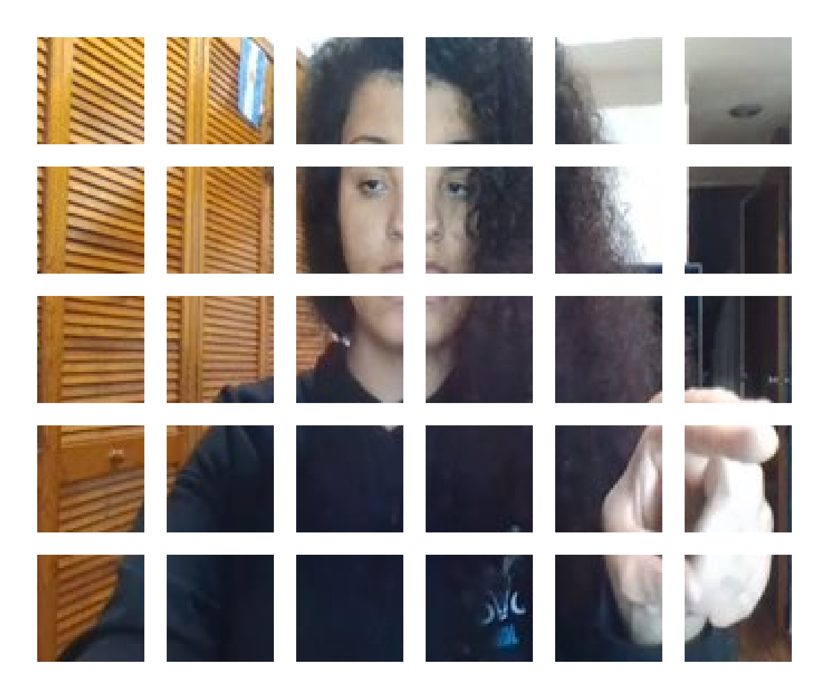
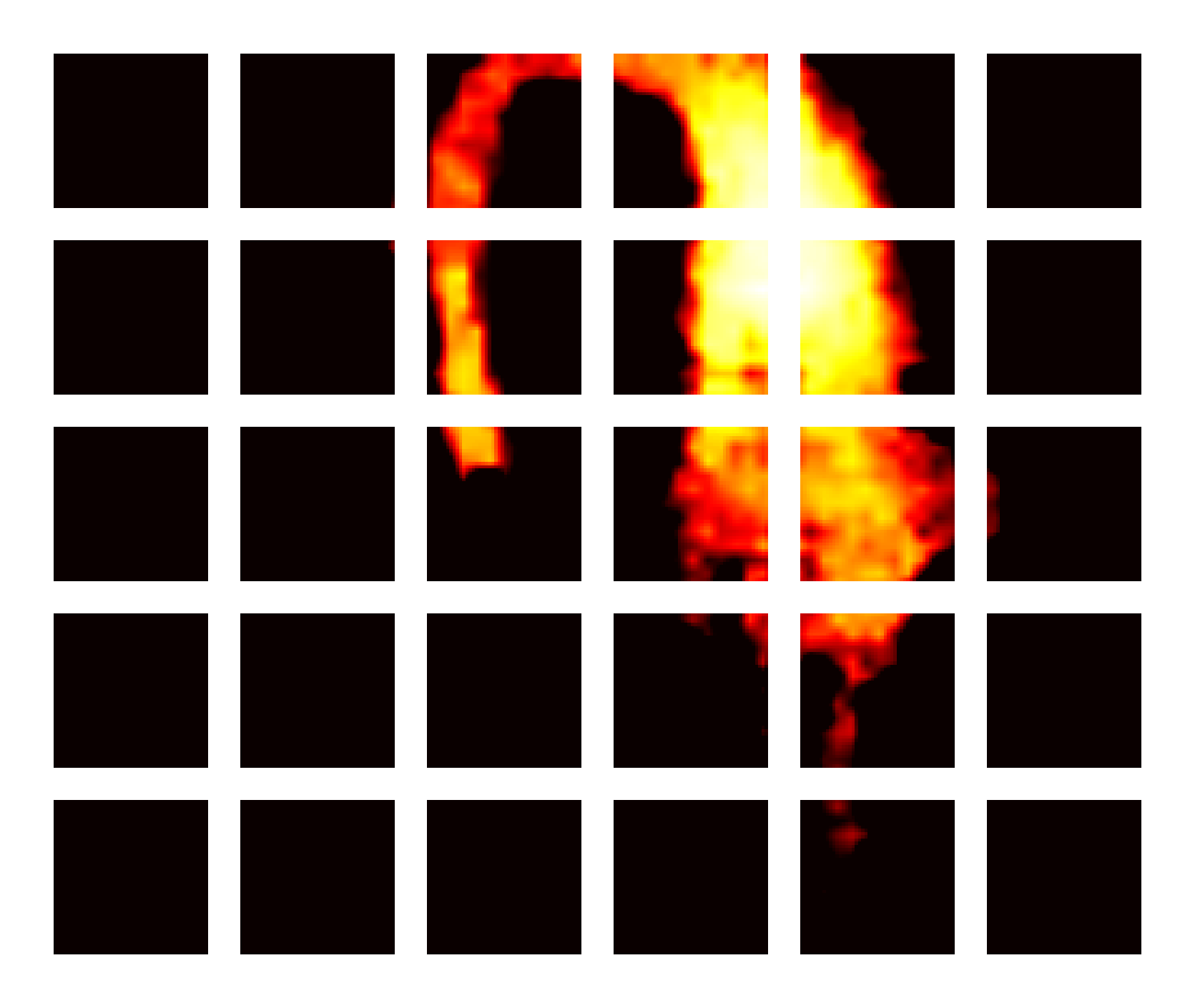
python visualize_qualitative/similarity_from_tempate_vis.py --image matcher/input/ipn2.jpg --descriptor output/descriptors/hair.pt

to load matcher/input/ipn2.jpg and match it with the hair descriptor in output/descriptors/.

Input Image	Saliency Map

Saliency Maps for each Dataset

The file matcher/similarity_from_template_for_dataset.py contains the necessary code to create the saliency maps for each dataset, which you need to precompute such that the training and evaluation of the methods presented in the paper works.

Again, make sure that the settings used in similarity_from_template_for_dataset.py are the same as in save_descriptor.py. Use the defaults if you want to reproduce our results from the paper.

The datasets have to be prepared as described in the Dataset section, and be placed/symlinked in data/.

Commandline Arguments

The usage of the file is identical to compute_similarities_from_descriptor.py with the addition of the dataset flag:

--dataset DATASET     options: [ 'ipn' | 'kth' | 'sbu' ]

To compute the necessary saliency maps for instance for IPN run:

python matcher/similarity_from_template_for_dataset.py -descriptorpath output/descriptors/mouth.pt -dataset ipn

This will populate data/ipn_mouth_sim/ with the similarity maps for the selected -descriptorpath file. Note that similarity_from_template_for_dataset.py can recover from partial completion and unfinished directories. It checks for the integrity of the processed files by comparing the number of images in the target directory for each sequence. No additional arguments are required, just run it again and it will continue where it left off.

To compute all the attributes for all the datasets you can reference matcher/run_batch.py.

Networks

We evaluate on a wide variety of models; the valid strings that identfy the models models/valid_models.py.

Each model communicates its required sampling of a video clip ($f \times r$) with the dataloader, and no additional configuration is required.

The following strings are valid ARCHITECTURE command line parameters for --architecture ARCHITECTURE

Privacy Classification Networks

resnet18
resnet50
resnet101
vit
vit_b_32

Action Classification Networks

x3d_s
x3d_m
x3d_l
slowfast_r50
slow_r50
i3d_r50
c2d_r50
csn_r101
r2plus1d_r50
mvit_base_16x4
e2s_x3d_s
e2s_x3d_m
e2s_x3d_l

Training & Evaluation

Training is straight forward; the logger found in simulation/ logs tensorboard entries and other data, and saves it so that it can later be read out and processed to create the tables for all the network architectures and modalities to be evaluated.

The evaluation code is almost identical to the training code and is also intended to be evaluated automatically by parsing the resulting tensorboard files.

We include the analysis file that produces correctly formatted latex tables with all the selected tensorboard files that are found in runs/, see Section Analysis.

The files that allow you to run the training and evalution are:

The command line parameters for all the afforementioned training and evaluation files is split into 3 groups Training, Evaluation, and Our Method. The ArgParse that is used for almost all files relating to network training and evaluation can be found in config.py.

Training

  --architecture ARCHITECTURE
  --datasetname DATASETNAME
  --weights_path WEIGHTS_PATH
  --num_epochs NUM_EPOCHS
  --num_workers NUM_WORKERS
  --batch_size BATCH_SIZE
  --num_frames NUM_FRAMES
  --lr LR
  -pretrained
  -train_backbone
  -privacy
  --gpus GPUS [GPUS ...]
  --accumulate_grad_batches ACCUMULATE_GRAD_BATCHES

Evaluation

  --masked MASKED
  --downsample DOWNSAMPLE
  --interpolation INTERPOLATION
  --blur BLUR
  --afd_combine_level AFD_COMBINE_LEVEL
  -combine_masked
  --downsample_masked DOWNSAMPLE_MASKED
  --interpolation_masked INTERPOLATION_MASKED
  -mean_fill

Our Method

  -selectively_mask
  --obfuscate OBFUSCATE [OBFUSCATE ...]
  -iid

To evaluate all the architectures that you want, it is straight forward to add or modify batch_train.py, and batch_eval.py.

The batch files just call the action / privacy files and set the command line parameters for multiple experiments.

Analysis

We try to provide all necessary files to reproduce the results if you decide to retrain all networks from scratch and evaluate them. The following analysis section highlights important files that are usefull to create ablations and visualize intermediate results.



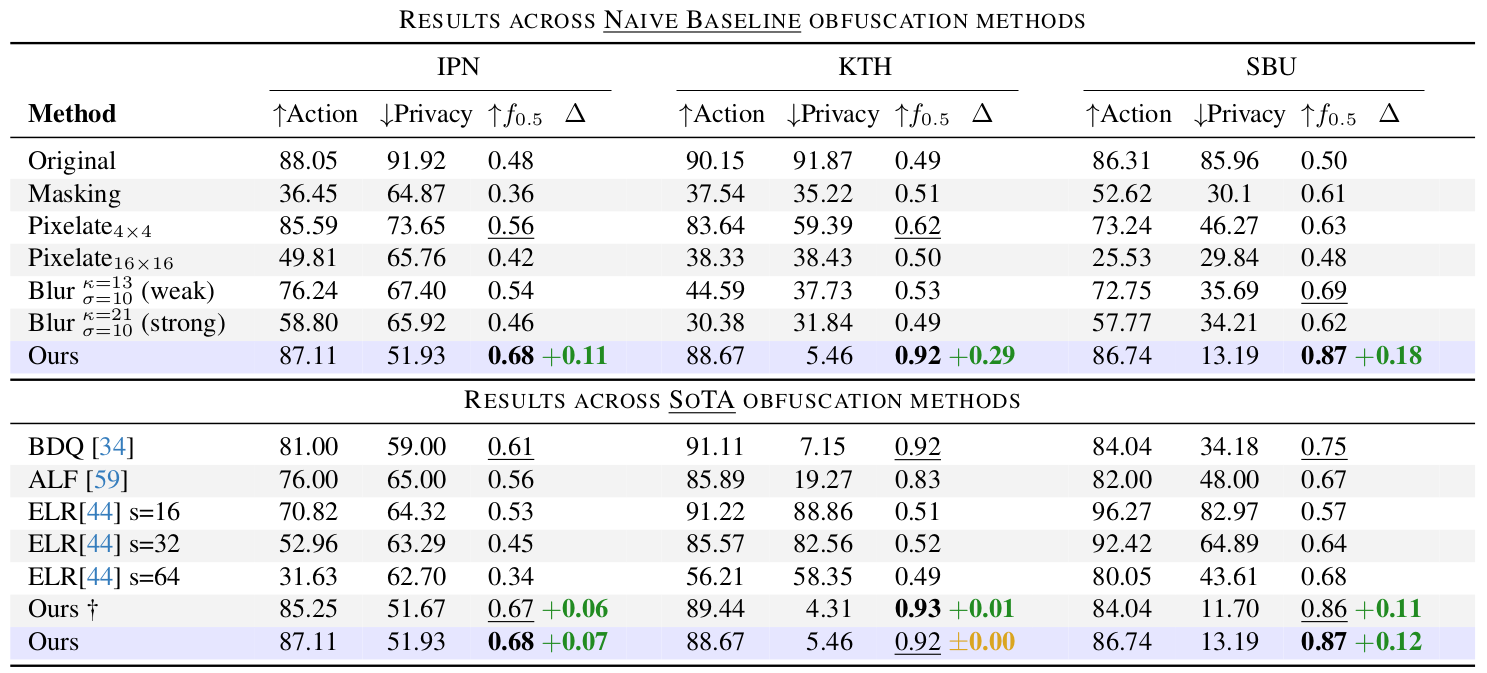`create_table_privacy.py` and `create_table_action.py`

There are additional files in ablation/ that were used to create ablations in Fig.5 and Fig.8 in the paper.

Ablation over the obfuscation performance of individual templates

`Fig5_ablate_individual_template.py`

The visualize_qualitative/, and visualize_quantitative/ directory contain files useful for qualitative analysis of baseline methods and the saliency matching based on selected templates.

Naive Baseline methods

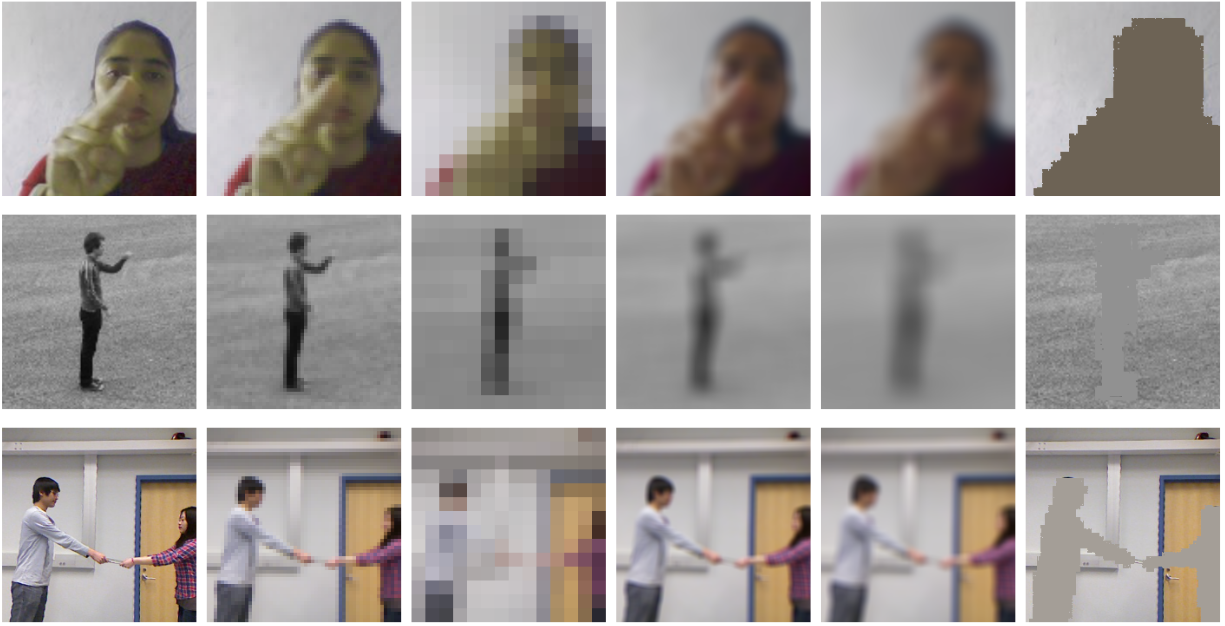`baselines_qualitative_vis.py`

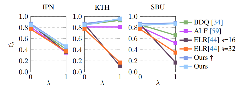
The average $f_{\lambda}$ value across all datasets can be plotted in $\LaTeX$-pgf with visualize_quantitative/Fig7_pgf_plots_average.py.

Additional ablation plots can be created as shown below:

Individual per dataset results	iid vs. Motion consistent Noise

`Fig7_pgf_plots_individual.py`	`Fig8_ablate_iidnoise_video_architecture.py`

Acknowledgements

Parts of this project use code from the following repositories:

Cite

@inproceedings{ilic2024selective,
  title={Selective, Interpretable and Motion Consistent Privacy Attribute Obfuscation for Action Recognition},
author={Ilic, Filip and Zhao, He and Pock, Thomas and Wildes, Richard P.},
  booktitle={Conference on Computer Vision and Pattern Recognition (CVPR)},
  year={2024}
}