This repository is for solving constrained optimization problems where objective and/or constraint functions are (arbitrary) PyTorch modules. It is mainly intended for optimization with pre-trained networks, but might be useful also in other contexts.
The algorithms in this package can solve problems of the form
    min  f(x)
    s.t. g(x) <= 0
         h(x) = 0
where f, g and h are locally Lipschitz functions.
Key functionalities of the package:
- forward and backward pass of functions can be done on GPU
- batched evaluation and Jacobian computation using PyTorch's
autograd; no gradient implementation needed - support for inequality and equality constraints; constraints can use only a subset of the optimization variable as input
- We have not (yet) extensively tested the solver on large-scale problems.
- The implemented solver is designed for nonsmooth, nonconvex problems, and as such, can solve a very general problem class. If your problem has a specific structure (e.g. convexity), then you will almost certainly get better performance by using software/solvers that are specifically written for the respective problem type. As starting point, check out
cvxpy. - The solver is not guaranteed to converge to a (global) solution (see the theoretical results in [1] for convergence to local solutions under certain assumptions).
The package is available from PyPi with
python -m pip install ncopt
Alternatively, for an editable version of this package in your Python environment, clone this repository and run the command
python -m pip install --editable .
The main solver implemented in this package is called SQP-GS, and has been developed by Curtis and Overton in [1]. See the detailed documentation.
The SQP-GS solver can be called via
    from ncopt.sqpgs import SQPGS
    problem = SQPGS(f, gI, gE)
    problem.solve()
Here f is the objective function, and gI and gE are a list of inequality and equality constraints. An empty list can be passed if no (in)equality constraints are needed.
The objective f and each element of gI and gE should be passed as an instance of ncopt.functions.ObjectiveOrConstraint (a simple wrapper around a torch.nn.Module).
- Each constraint function is allowed to have multi-dimensional output (see example below).
- IMPORTANT: For the objective, we further need to specify the dimension of the optimization variable with the argument
dim. For each constraint, we need to specify the output dimension withdim_out.
For example, a linear constraint function Ax - b <= 0 can be implemented as follows:
    from ncopt.functions import ObjectiveOrConstraint
    A = ..                      # your data
    b = ..                      # your data
    g = ObjectiveOrConstraint(torch.nn.Linear(2, 2), dim_out=2)
    g.model.weight.data = A    # pass A
g.model.bias.data = -b # pass bLet's assume we have a torch.nn.Module, call it model, which we want to use as objective/constraint. For the solver, we can pass the function as
f = ObjectiveOrConstraint(model)
-
Dimension handling: Each function must be designed for batched evaluation (that is, the first dimension of the input is the batch size). Also, the output shape of
modelmust be two-dimensional, that is(batch_size, dim_out), wheredim_outis the output dimension for a constraint, anddim_out=1for the objective. -
Device handling: The forward pass, and Jacobian calculation is done on the device on which the parameters of your model. For example, you can use
model.to(device)before creatingf. See this Colab example how to use a GPU. -
Input preparation: Different constraints might only need a part of the optimization variable as input, or might require additional preparation such as reshaping from vector to image. (Note that the optimization variable is handled always as vector). For this, you can specify a callable
prepare_inputwhen initializing aObjectiveOrConstraintobject. Any reshaping or cropping etc. can be handled with this function. Please note thatprepare_inputshould be compatible with batched forward passes.
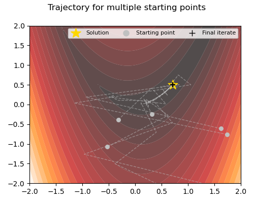
This example is taken from Example 5.1 in [1] and involves minimizing a nonsmooth Rosenbrock function, constrained with a maximum function. The picture below shows the trajectory of the SQP-GS solver for different starting points. The final iterates are marked with the black plus while the analytical solution is marked with the golden star. We can see that the algorithm finds the minimizer consistently.
This example is taken from Example 5.3 in [1]. We minimize the q-norm
When
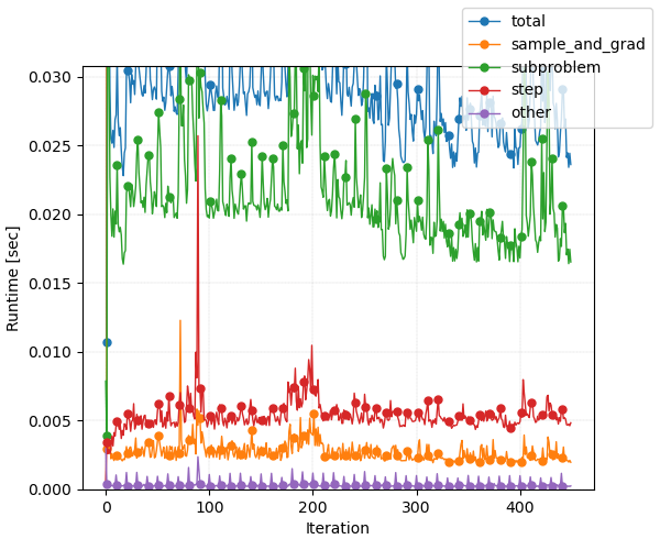
This problem has dimension 256, with one scalar constraint. To give a feeling for runtime, below is the runtime per iteration (for sample_and_grad), solve the quadratic subproblem (subproblem), do the update step of iterate and approximate Hessian (step), and all other routines.
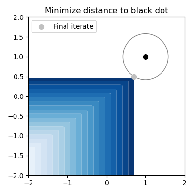
This toy example illustrates how to use a pretrained neural network as constraint function in ncOPT. We train a simple model to learn the mapping
Below we show the feasible set (in blue), and the final iterate, if we use as objective the squared distance to the vector of ones.
[1] Frank E. Curtis and Michael L. Overton, A sequential quadratic programming algorithm for nonconvex, nonsmooth constrained optimization, SIAM Journal on Optimization 2012 22:2, 474-500, https://doi.org/10.1137/090780201.


