fabiana001/paysim_analysis

Exploratory Data Analysis of PaySIM dataset

Transaction Fraud Detection

Fraud is a global economic menace which threatens the survival of individuals, firms, industries and economies, and the mobile money service is no exception. In this analysis we explore a synthetic dataset, related to a mobile money service. Our goal is to investigate the performance of machine learning models on a highly skewed dataset.

1 Overview

Financial Fraud detection systems are challenging due two major reasons: i) fraudulent behaviors can follow different schemas; ii) fraudulent transactions are very rare.

In this analysis we focus on the PaySIM [1] dataset. It is a synthetic dataset constructed using an agent based simulation approach [2]. In particular, PaySim simulates mobile money transactions based on a sample of real transactions extracted from the logs of a mobile money service implemented in an African country.

The analysis is structured as follows: Section 2. presents an explorative analysis of the dataset; Section 3. focuses on data enrichment, dimensionality reduction and data transformation; Section 4. addresses the unbalanced dataset problem; Section 5. compares performances of a SVM classifier on different dataset configurations

Exploratory Data Analysis

The dataset contains 6.362.620 transactions. Only 8213 transactions are labeled as fraudulent (i.e. 0.1%).

There are 6.589.578 unique clients. Most clients do one transaction per month and only few than 1% of clients transact more. Moreover, each defrauded clients has at most one transaction labeled as fraud. This means that the dataset doesn't contain complex schemas of frauds.

Fraudulent transactions can be only of type CASH-OUT (4116 transactions) and TRANSFER (4097 transactions). Therefore, frauds can be a one shot transfer to a mule account or a single withdrawal cash from a merchant. For this reason, the mean amount of fraudulent transactions is higher than the mean of normal transactions.

The following figure shows the distribution of transactions, when type is CASH-OUT or TRANSFER. The value True means that type is CASH-OUT, while the value False means that type is TRANSFER.

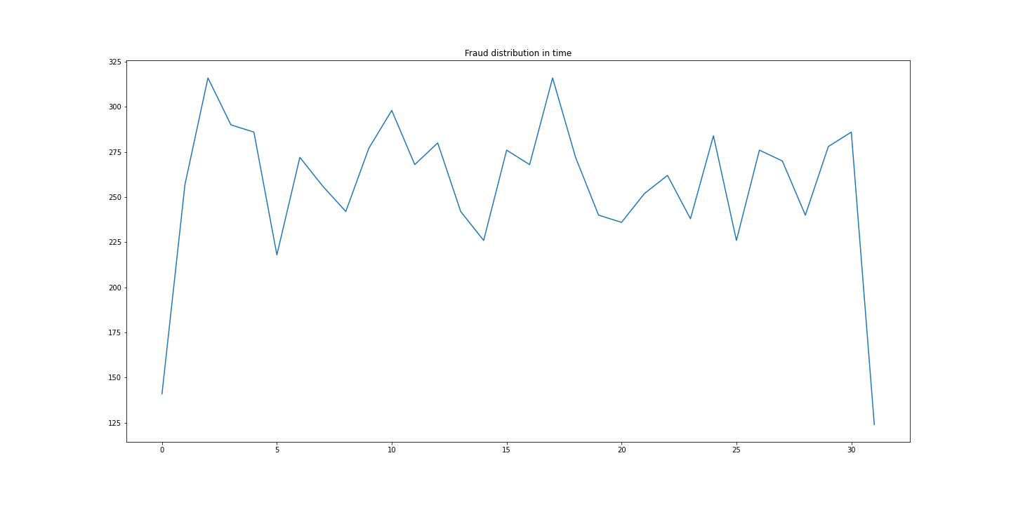
Fraudulent transactions are equally distributed at the time. There are an average of 256 fraudulent transactions per day (11 per hour). The highest peaks are at days 2, 10 and 17.

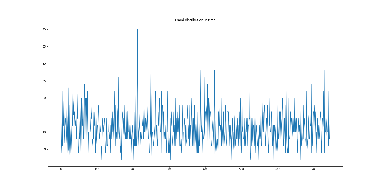
If we aggregate per hour, it is possible to see that frauds are still equally distributed. The highest peak is at step 212 (day 9) with 40 transactions.

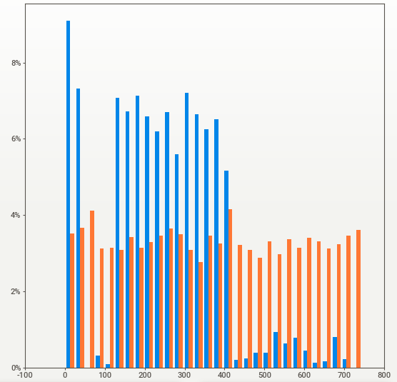
However, if we compare the average number of normal and fraud transactions per step, we can see a different data distribution. In particular, normal transactions are not equally distributed, but they are more concentrated on the first fifteen days.

About 32% of transactions have both fields oldbalanceOrg and newbalanceOrig equal to zero. Maybe those transactions are not accepted by the system or negative balances are set to 0. The same phenomenon is present in the fields oldbalanceDest and newbalanceDest.

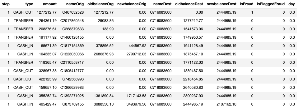
Moreover, if we analyze the fields oldbalanceDest and newbalanceDest of clients (merchants) having multiple incoming transactions, it is possible to note that there doesn't exist a correlation between these attributes. If we consider for example all incoming and outgoing transactions for client C716083600 at step 1, the value of oldbalanceDest changes for each transaction. The same is not for the newbalanceDest, that is always the same except for the last row.

A complete report on univariate and bivariate analysis can be found here.

3 Dataset Manipulation

3.1 Data Enrichment

We enrich each transaction with information about the spending behaviour of source and destination clients: the number of outlinks of a client (inlink of a merchant); the average amount of client outlinks (merchant inlinks).

In particular, we add the following features:

• countOrigStep:number of outgoing transactions made by nameOrig at step
• countOrig: number of outgoing transactions made by nameOrig
• countDestStep: number of incoming transactions received bynameDest at step
• countDest: number of incoming transactions received bynameDest
• avgAmtOrigStep: average amount of outgoing transactions made bynameOrig at step
• avgAmtOrig: average amount of outgoing transactions made by nameOrig
• avgAmtDestStep: average amount of incoming transactions received bynameDest at step
• avgAmtDest: average amount of of incoming transactions received bynameDest
• is_CASH_OUT: is True if type is CASH_OUT

3.2 Dimensionality Reduction

We remove all data records having the following properties:

• The transaction type is DEBIT and CASH_IN;
• nameDest starts from M.

The filtered dataset is composed of 2.770.409 data records. It represents 43% of the whole dataset.

3.3 Feature Scaling

Feature Scaling makes sure that the features of the data-set are measured on the same scale. We apply z-score normalization to all numeric features related to the transactions amount and the number of outlinks/inlinks of a client

3.4 Feature Selection

The final dataset is composed by the features described in Section 3.1 and the following original features:

• step;
• amount;
• oldbalanceOrg;
• newbalanceOrg;
• oldbalanceDest;
• newbalanceDest;
• avgAmtOrigStep;

All numerical features will be scaled through Z-score normalization.

Handling Unbalanced Dataset

The main challenge of Financial Fraud Detection is that datasets are highly skewed. The performance of a detection model is greatly affected by the sampling approach on the dataset.

In this analysis we focus on some state-of-art approach.

Undersampling

Undersampling techniques remove examples from the training dataset that belong to the majority class in order to better balance the class distribution, such as reducing the skew from a 1:100 to a 1:10, 1:2, or even a 1:1 class distribution. The main drawback of undersampling is the information loss due the reduction of data points.

We apply two undersampling approaches: Tomek Links, NearMiss.

Tomek Links

Undersampling through Tomek links [4] consists in removing the instances of the majority class in the way to increase the space between the two classes, facilitating the classification process.

In our case, Tomek Links Undersampling removes only 1000 of data records.

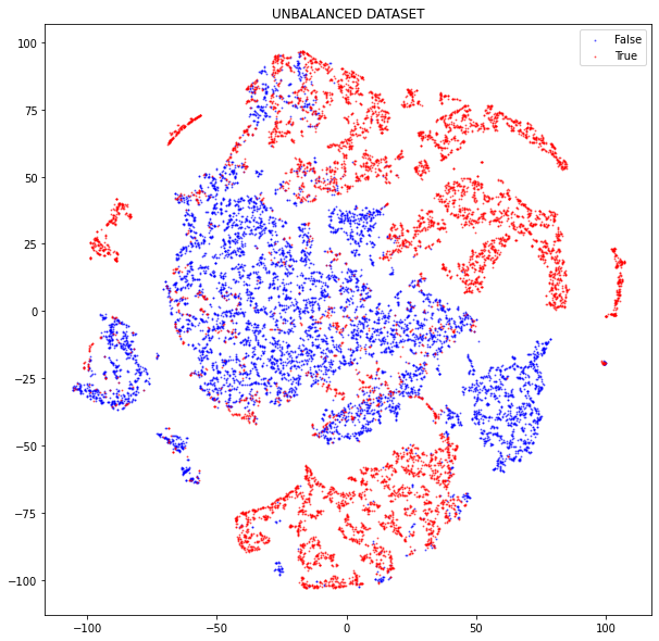
The figure below shows a visual representation of the input dataset. The image plots all frauds, and a sample of 8.000 data points of the majority class. The 2D representation is obtained by applying TSNE ( t-Distributed Stochastic Neighbor Embedding).
We can note that data belonging to the same class is close together, and in this space data is easily separable.

Near Miss Undersampling

Use KNN to select the most representative data points. There are three different types of sampling:

• NearMiss1: selects the examples from the majority class having the smallest average distance from three closest examples of minority class.
• NearMiss2: selects the examples from the majority class having the smallest average distance from three farthest examples of minority class.
• NearMiss3: for each example of minority class, a sample of closest examples of majority class is extracted (to be sure that all positive points are surrounded by some negative example).

The figure below shows a visual representation of the sampled dataset with NearMiss3.

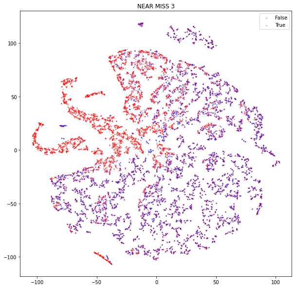
Unlike the previous figure, it is difficult to identify clusters of data belonging to the same class.

Oversampling

Unlike Undersampling, oversampling algorithms increase the size of the minority class.

Oversampling does not increase information but, it does increase the the misclassification cost of the minority examples. As drawback it increases the likelihood of overfitting since it replicates the minority class events.

SMOTE

SMOTE generates examples based on the distance of each data (usually using Euclidean distance) and the minority class nearest neighbors, so the generated examples are different from the original minority class.

In short, the process to generate the synthetic samples are as follows.

• Choose random data from the minority class.
• Calculate the Euclidean distance between the random data and its k nearest neighbors.
• Multiply the difference with a random number between 0 and 1, then add the result to the minority class as a synthetic sample.
• Repeat the procedure until the desired proportion of minority class is met.

The original paper on SMOTE suggested combining SMOTE with random undersampling of the majority class.

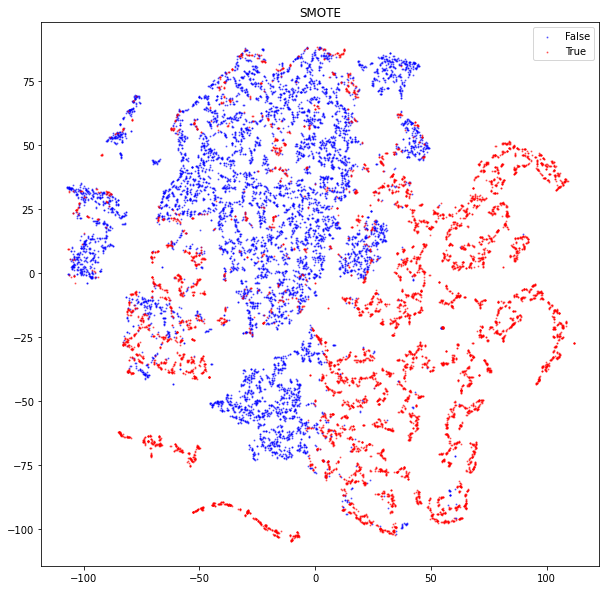
The following figure shows a visual representation of a sample extracted using smote. Plotted data is a sample of 16.000 data points equally sampled between the two classes. Although there are regions where both positive and negative examples are close together, it is still possible to identify homogeneous clusters wrt our label.

Hybrid Sampling

Hybrid algorithms combine both undersampling and oversampling. In our analysis, like the SMOTE authors suggest, we apply the following hybrid approach:

- Random undersampling (200.000 data points)
- Smote oversampling

In this way we obtain a balanced sample of size 400.000

Classification Algorithms

Since our goal is to analyze how the performances of a Machine Learning model change varying the sample approach, we will consider the following cases:

• SVM on balanced dataset
• SVM on unbalanced dataset, forcing the model to penalize mistakes on the minority class by an amount proportional to how underrepresented it is.
• One Class SVM fitted on a random sample of the majority class.

Unlike a standard SVM, One Class SVM is fit in an unsupervised manner and does not provide the normal hyperparameters. Instead, it provides a hyperparameter nu that controls the sensitivity of the support vectors and should be tuned to the approximate ratio of outliers in the data.

A SVM is a machine learning model that finds a hyperplane in an N-dimensional space (N — the number of features) that distinctly classifies the data points. Among all possible hyperplanes, SVM learns the hyperplane having the maximum margin, i.e the maximum distance between data points of both classes.

SVM works relatively well when there is a clear margin of separation between classes. However, if data points are not linearly separable, kernel functions can be used. A Kernel function is a similarity function that measures the distance of data points into a feature space with higher dimension. Data points in this feature space are linearly separable. For time reasons, applying kernel functions on SVM and comparing performances is out of scope of the analysis.

Results

For a time reason, we apply 10 Cross Validation only to the SVM trained on the undersampled dataset with NearMiss3. In all the other cases, we split the input dataset in the Training set (70%) and Testing Set (30). Sampling is stratified wrt isFraud feature to be sure that classes are equally represented.

Metrics

• Recall (True Positive Rate) computes the percentage of correctly identified frauds;
• Precision that is the proportion of TP over the transactions ranked as frauds;
• F1 score : harmonic mean between precision and recall;
• Matthews correlation coefficient (MCC): measures the quality of the detection rate in terms of the correlation coefficient between the observed and predicted classifications (ranking); a coefficient of +1 represents a perfect ranking, 0 no better than random prediction and −1 indicates total disagreement between prediction and observation. MCC produces a more informative and truthful score in evaluating binary classifications of unbalanced datasets.
• ROC AUC score that express the ratio between the TPR and the FPP
• training time in seconds.

A Good financial fraud model should be characterized by:

• a low False Negative Rate, since fraudulent transactions increase the operative risk of the money service company.
• a low False Positive Rate, since we want to block only fraudulent transactions without blocking the normal operativity of the client.

Results

The following figure shows the performances of a SVM model learned on different dataset configurations:

• SVM on unbalanced DF (2M): the SVM is learned on the whole dataset but a higher misclassification cost is given to the minority class.
• SVM on SMOTE DF (400k): The input dataset is sampled using an hybrid approach. First the majority class is randomly undersampled (200k), then new data points of the minority class are generated using SMOTE. The final balanced dataset is composed of 400k elements.
• SVM on NearMiss3 (16k): The input dataset is undersampled using the NearMiss3 algorithm. The final balanced dataset is composed of 16k data points.
• One Class SVM (200k): The majority class is randomly sampled (200k). The model is learned using only the majority class. The test set is composed of 16k data points equally distributed between the two classes.

| Metrics             | SVM on unbalanced DF (2M) | SVM on SMOTE DF (400k) | SVM on NearMiss3 (16k) | One Class SVM (200k) |
|---------------------|---------------------------|------------------------|------------------------|----------------------|
| Precision           | 0.55                      | 0.92                   | 0.80                   | 0.77                 |
| Recall              | 0.93                      | 0.92                   | 0.78                   | 0.66                 |
| F1                  | 0.59                      | 0.92                   | 0.77                   | 0.61                 |
| MCC                 | 0.29                      | 0.83                   | 0.58                   | 0.41                 |
| ROC AUC             | 0.93                      | 0.98                   | 0.85                   | 0.66                 |
| training time (sec) | 540                       | 64                     | 1.4                    | 780                  |

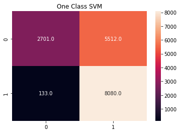
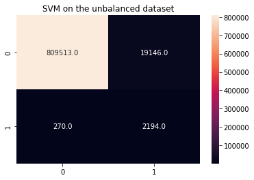
One Class SVM and SVM on unbalanced DF have the worst performances. However, for time reasons we have not applied Cross Validation. Therefore, performance scores may not be reliable. Although they have a comparable F1 score, One Class SVM is characterized by an higher False Positive rate (i.e. 0.67 wrt 0.02); SVM on unbalanced DF is characterized by an higher False Negative Rate (i.e. 0.10 wrt 0.02).

The figures below show the confusion matrix of One Class SVM and SVM on unbalanced DF

The best performances are obtained by SVM on SMOTE and SVM on NearMiss3. Performance scores are the mean of scores obtained through 10-Cross Validation. It is possible that the high performances of SMOTE are due to the fact that positive examples in the test set are very similar to those in the training set. As future work, it is interesting to use as a positive test set, examples that are not used in the data oversampling step. Performances on this test set should be more truthful.

The performances in SVM on NearMiss3 are very interesting, since negative examples are very similar to the positive ones. As future work, we can compare the performances of non linear models (e.g. SVM with kernel) and analyze more sophisticated algorithms, such as Autoencorders or Self Supervised Learning.