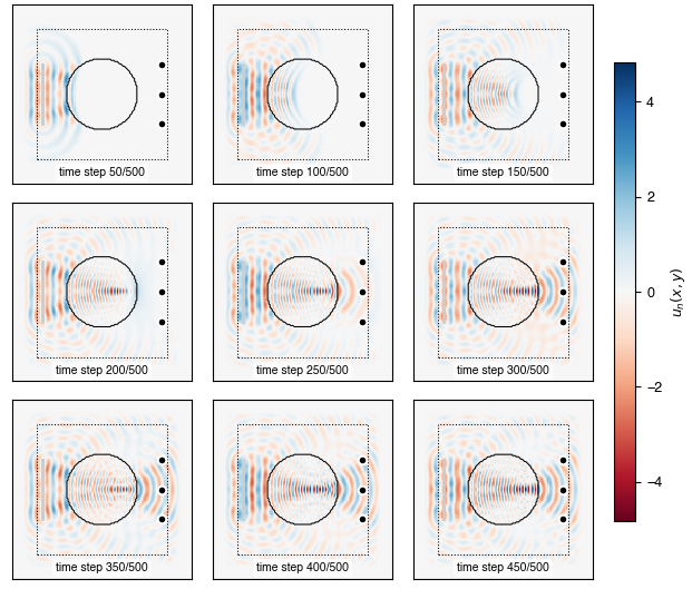
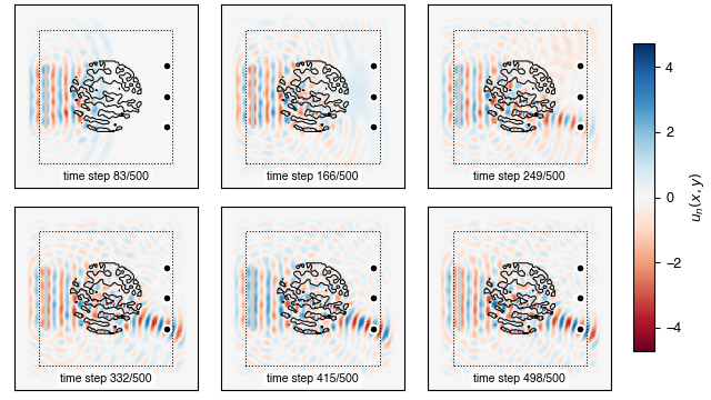
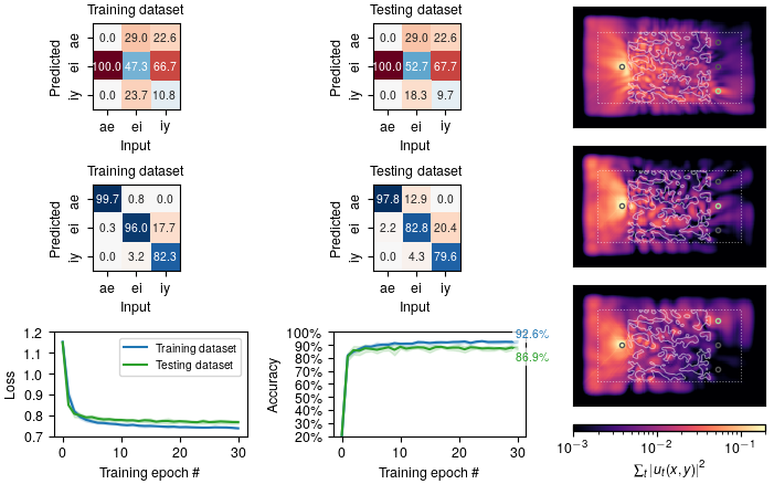
This python package provides recurrent neural network (RNN) modules for pytorch that compute time-domain solutions to the scalar wave equation. The code in this package is the basis for the results presented in our recent paper, where we demonstrate that recordings of spoken vowels can be classified as their waveforms propagate through a trained inhomogeneous material distribution.
This package not only provides a numerical framework for solving the wave equation, but it also allows the gradient of the solutions to be computed automatically via pytorch's automatic differentiation framework. This gradient computation is equivalent to the adjoint variable method (AVM) that has recently gained popularity for performing inverse design and optimization of photonic devices.
For additional information and discussion see our paper:
- T. W. Hughes*, I. A. D. Williamson*, M. Minkov, and S. Fan, Wave physics as an analog recurrent neural network, Science Advances, vol. 5, no. 12, p. eaay6946, Dec. 2019
The machine learning examples in this package are designed around the task of vowel recognition, using the dataset of raw audio recordings available from Prof James Hillenbrand's website. However, the core modules provided by this package, which are described below, may be applied to other learning or inverse design tasks involving time-series data.
The wavetorch package provides several individual modules, each subclassing torch.nn.Module. These modules can be combined to model the wave equation or (potentially) used as components to build other networks.
WaveRNN- A wrapper which contains one or moreWaveSourcemodules, zero or moreWaveProbemodules, and a singleWaveCellmodule. TheWaveRNNmodule is a convenient wrapper around the individual components and handles time-stepping the wave equation. If no probes are present, the output ofWaveRNNis the scalar field distribution as a function of time. If probes are present, the output will be (by default) the probe values, but this output can be overridded to instead output the field distribution.WaveCell- Implements a single time step of the scalar wave equation.WaveGeometry- The children of this module implement the parameterization of the physical domain used by theWaveCellmodule. Although the geometry module subclassestorch.nn.Module, it has noforward()method and serves only to provide a parameterization of the material density to theWaveCellmodule. Subclassingtorch.nn.Modulewas necessary in order to properly expose the trainable parameters to pytorch.
WaveSource- Implements a source for injecting waves into the scalar wave equation.WaveProbe- Implements a probe for measuring wave amplitudes (or intensities) at points in the domain defined by aWaveGeometry.
To train the model using the configuration specified by the file study/example.yml, issue the following command from the top-level directory of the repository:
python ./study/vowel_train.py ./study/example.yml
The configuration file, study/example.yml, is commented to provide information on how the vowel data is processed, how the physics of the problem is specified, and how the training process is configured.
During training, the progress of the optimization will be printed to the screen. At the end of each epoch, the current state of the model, along with a history of the model state and performance at all previous epochs and cross validation folds, is saved to a file.
WARNING: depending on the batch size, the window length, and the sample rate for the vowel data (all of which are specified in the YAML configuration file) the gradient computation may require a significant amount of memory. It is recommended to start small with the batch size and work your way up gradually, depending on what your machine can handle.
A summary of a trained model which was previously saved to disk can be generated like so:
python ./study/vowel_summary.py <PATH_TO_MODEL>
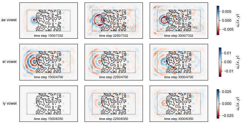
Snapshots of the scalar field distribution for randomly selected vowels samples can be generated like so:
python ./study/vowel_analyze.py fields <PATH_TO_MODEL> --times 1500 2500 3500 ...
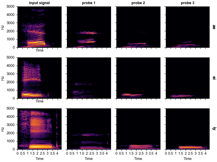
A matrix of short time Fourier transforms of the received signal, where the row corresponds to an input vowel and the column corresponds to a particular probe (matching the confusion matrix distribution) can be generated like so:
python ./study/vowel_analyze.py stft <PATH_TO_MODEL>
pytorchscikit-learnscikit-imagelibrosaseabornmatplotlibnumpyyamlpandas

