Vehicle Detection Project
The goals / steps of this project are the following:
- Perform a Histogram of Oriented Gradients (HOG) feature extraction on a labeled training set of images and train a classifier Linear SVM classifier
- Optionally, you can also apply a color transform and append binned color features, as well as histograms of color, to your HOG feature vector.
- Note: for those first two steps don't forget to normalize your features and randomize a selection for training and testing.
- Implement a sliding-window technique and use your trained classifier to search for vehicles in images.
- Run your pipeline on a video stream (start with the test_video.mp4 and later implement on full project_video.mp4) and create a heat map of recurring detections frame by frame to reject outliers and follow detected vehicles.
- Estimate a bounding box for vehicles detected.
In the project directory, type:
python3 main.py --input <video_clip>
where <video_clip> is the name of the file with the video clip to be processed. If not provided, it defaults to project_video.mp4
car-no-car-*.ppickled files with labeled dataset images.classifier.ppickled file with trained classifier and scaler.extract.pyutility program to extract a random sample of car images from Udacity's Annotated Driver Dataset..gitignoreGIT configuration file.main.pythe program for vehicle detection.output_images/pictures showed in thisREADME.mdproject_video.mp4the test video clip.project_video-out.mp4the processing output, with detected vehicles.README.mdthis file, the project write-up.requirements.txtlist of dependencies formain.pytest_images/video frames useful for parameters tuning and debugging.
Rubric Points
Here I will consider the requirements individually and describe how I addressed each one in my implementation.
This is it!
1. Explain how (and identify where in your code) you extracted HOG features from the training images.
The main() function tries to load the dataset from a pickled file car-no-car.p. If it doesn't find it, then it loads the dataset images, and pickles them along with their labels calling load_and_pickle_datasets(). The dataset has been obtained from:
- GTI Vehicle Image Database
- KITTI Vision Benchmark Suite
- Udacity's Annotated Driving Dataset
main() shuffles and splits the dataset between a training set (90%) and a validation set (10%) calling shuffle_and_split_dataset(). It then calls fit_and_pickle_classifier(), which extracts features from the dataset images before fitting a classifier.
I adopted OpenCV implementation of HOG, cv2.HOGDescriptor(), finding it faster than scikit-image implementation, skimage.feature.hog(). It also allows tuning some additional parameters.
Function get_hog_descriptor() initializes parameters for the HOG, and function compute_hog_features() extracts and returns HOG features for a given image. It can operate on a single channel image, or a 3 channels image.
Function compute_histogram_features() returns concatenated color and tone histogram features for a given image and choice of image channels.
Function compute_image_features() concatenates and returns HOG and color histogram features for a given image, not scaled. After numerous experiments, I settled for a features descriptor that concatenates:
- a HOG for the V channel of the image in HSV color space;
- a color histogram (16 bins each) for the U and V channels of the image in YUV color space.
Images, before being used to train and validate the classifier and for detection, are all resized to 64x64 pixels.
To compute the HOG, I used a cell size of 8x8 pixels, a block size of 2x2 cells, a stride for blocks of 8x8 pixels (i.e. 1 cell), 16 bins, gamma correction and signed gradient.
I started with 9 bins and unsigned gradient, based on Dalal and Triggs paper on pedestrians detection, but then found that increasing the number of bins to 16 and adopting a signed gradient increased drastically the detection of true positives in video frames.
I had three ways to test and tune parameter values, for HOG and other stages of the pipeline: testing the classifier on a validation dataset, testing detection on selected camera frames, and testing detection on the whole input video clip. The latter is the most time consuming, and could only be done after the pipeline was completely implemented.
I tuned parameters by trial and error first running the trained classifier on a validation set I sampled, until further tweaking didn't bring about significant improvements, and then on frames I selected from the input video clip. Test on video frames was subjective.
3. Describe how (and identify where in your code) you trained a classifier using your selected HOG features (and color features if you used them).
Function fit_and_pickle_classifier() re-scales image features with sklearn.preprocessing.StandardScaler, which results in improved detection accuracy. It then fits a Support Vector Machine (SVM) linear classifier with sklearn.svm.LinearSVC¶(), evaluates the result on the validation set, and saves scaler and classifier in a pickled file. At the next run, it will load them from the pickled file and avoid repeating the computation.
I set the C parameter for the Linear SVM classifier to 0.001 by trial and error, based on the classifier performance on the validation set. I didn't find a very fine tuning worthwhile, perhaps based on a grid search. Comparing performance on the validation set and camera frames, I could see I was just overfitting my training data; improvements on validation performance rom 98% to 99% didn't reflect on improved detection in video frames.
Overall accuracy of the trained classifier on the validation set is 0.980. Here below a table with details of validation performance; Class 1 corresponds to cars, and Class 0 to no-cars.
| Class | Precision | Recall | F-score | Support |
|---|---|---|---|---|
| 0 | 0.983 | 0.986 | 0.985 | 2278 |
| 1 | 0.974 | 0.968 | 0.971 | 1190 |
When using validation to tune parameters, I tried to obtain a validation accuracy as high as possible, while maintaining precision and recall for both classes above 0.95 and, most important, solid (if subjective) detection of cars in video frames.
1. Describe how (and identify where in your code) you implemented a sliding window search. How did you decide what scales to search and how much to overlap windows?
Class Perspective_grid is a Python generator that yields coordinates for a sliding window. Using it as an iterator, it provides a succession of sliding window coordinates that cover the region of interest (ROI) in the image, in a certain pattern. The ROI goes from where the horizon should be down to the bottom of the screen. Windows have size of 128x128 pixels and 192*192 pixels, and windows of the same size overlap each other by 75%. Smaller windows cover the ROI closer to the horizon, while larger windows cover it closer to the bottom of the screen.
Initially I had adopted also windows of size 64x64 pixels and 256x256 pixels. However, those two sizes didn't make a difference in detecting cars in the project_video.mp4 clip; I therefore did without, speeding-up computation. Decreasing overlapping from 75% to 50% made the coputation faster but also made detection less reliable.
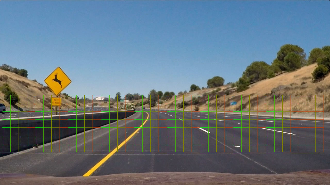
I wrote a function display_image_with_windows() that draws the sliding windows in different colors over an image of choice, to help tune positions, scale and overlap. Image below shows overlapping sliding windows with a size of 128x128 pixels; one window in the image is made by 4x4 squares in the grid.
2. Show some examples of test images to demonstrate how your pipeline is working. What did you do to optimize the performance of your classifier?
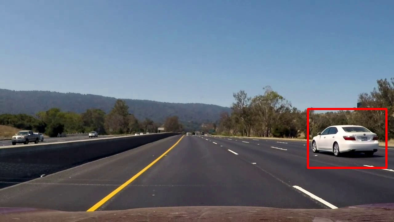
In spite of the parameters tuning, that could give me a validation accuracy up to 99%, detection was often missing the white car, prominent on the right side of sevaral test frames. Detection was week for both cars, but especially the white one, with few or no sliding windows detecting them in each frame. As a consequence, cars in the heatmap couldn't be differentiated from false positives; any thresholding that would remove a significant amount of false positives would also remove the cars!
Increasing the number of HOG bins to 16 and adding color histograms to features helped, but not enough. Exploring the dataset, I could see that few images had the car from the perspective seen for the white car. Also, most dataset images were tightly cropped, not showing the entire car silhouette. I believe that can help limiting false positives, as the image doesn't include lane lines, curbs, signs, etc.; but it also prevents the classifier from learning the car outline, a conspicuous HOG feature.
I decided I need a larger dataset. To do so, I wrote a short program to extract car images from one of Udacity's Annotated Driver Datasets. This is comprised of frames taken in order by a camera; I picked images randomly among all available images, to reduce the probability that chosen images were in a tight time series.
Writing code to extract non-car images from Udacity's dataset would have been more time consuming, I decided instead to augment the dataset already in use, adding to it a left-to-right flipped copy of every non-car image.
With the additional images in the dataset, accuracy of validation went down from 99% to 98%, while detected cars in the heatmap were more prominent, with a stronger signal than many false positives.
Detection still picked up recurrent false positives along the edges of the road, and in the middle of the lane, often enough for them to compete with detected cars in the heatmap. To get rid of them I went for hard negatives mining, identifying and adding to the dataset portions of the frame that were giving frequent false positives. Below a sample of the added images.
 |
 |
 |
|---|---|---|
 |
 |
 |
 |
 |
 |
After the hard negative mining, I could finally determine a threshold for the heatmap that successfully discriminates detected cars from the remaining false positives.
The initial dataset had 2826 car and 17936 non-car images. The expanded dataset contains 11999 car and 45344 non-car images, after non-car image augmentaton.
1. Provide a link to your final video output. Your pipeline should perform reasonably well on the entire project video (somewhat wobbly or unstable bounding boxes are ok as long as you are identifying the vehicles most of the time with minimal false positives.)
Here's a link to my video result
2. Describe how (and identify where in your code) you implemented some kind of filter for false positives and some method for combining overlapping bounding boxes.
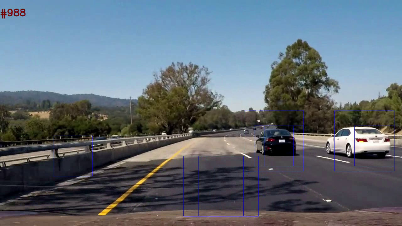
Function main() initialises a heatmap to all zeros (black) before it starts looping over the input video frames. For every frame, it detects probable bounding boxes of cars calling find_bounding_boxes(), drawn in blue in the video frame below.
Next, main() uses the result to have the heatmap updated, calling update_heat_map().
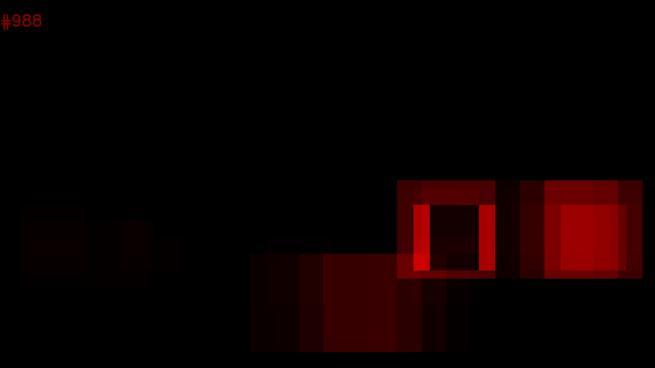
For every bounding box, function update_heat_map() increases, by a set amount, every pixel in the heatmap inside the bounding box; it then averages the heatmap across the last 15 frames, to smooth the resulting detection; finally, it makes a copy of the heatmap where pixels below a set threshold are zeroed, while remaining pixels are rounded to the nearest integer value. The image below is the heatmap before thresholding.
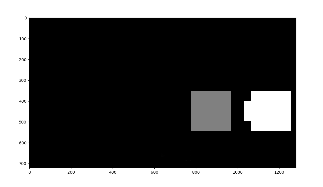
Function main() uses the thresholded heatmap to determine bounding boxes for cars: it calls scipy.ndimage.measurements.label() to enumerate clusters of adjacent non-zero pixels from the thresholded heatmap. Below a graphic representation of label()'s output.
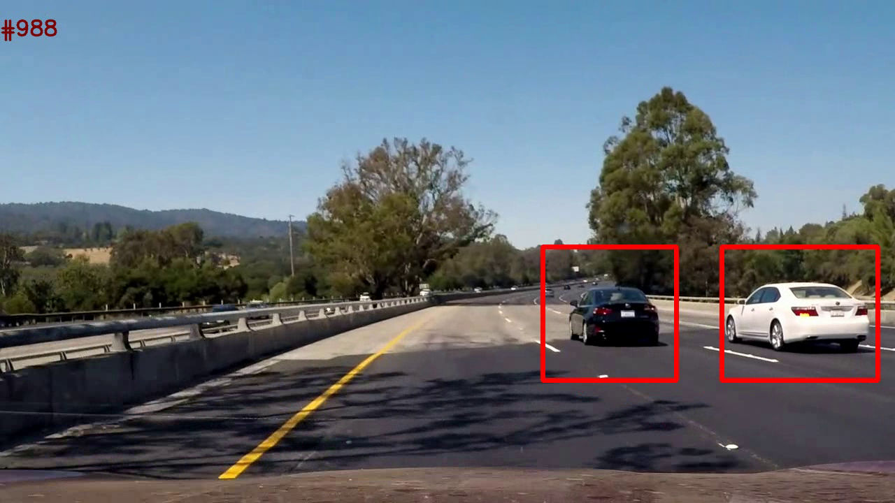
Finally, main() determines the tightest (smallest) bounding box for every cluster, calling function draw_labeled_bounding_boxes() (adopted from Udacity's lesson). The frame below is an example of the result, saved into the output video stream.
1. Briefly discuss any problems / issues you faced in your implementation of this project. Where will your pipeline likely fail? What could you do to make it more robust?
I could reach an accuracy on the validation set of up to 99% and still have detection miss cars in video frames, and give plenty of false positives. In the heatmap, cars were not distinguishable from false positive, having comparable intensities.
Detection would often miss the white car, and catch false positives, especially along the top of guardrails and in the middle of the lane, catching between the lane line markers.
Overfitting may have been an issue, but it seemed to me the dataset was insufficient. I therefore went for more training data, extracting a random sample of images from Udacity's annotated driving dataset. That, combined with a proper choice of features extracted from images, allowed to have a solid detection of cars in the input video clip.
False positives were still an issue. I mined the "hard negatives" and added them to the dataset, lowering the rate of false pasitives to the point that I could successfully threshold the heatmap, telling apart cars from non-car.
A better solution would be to select also negatives (non-cars) from Udacity's annotated driving dataset, more time-consuming but more robust.
The program processes an input video at around 6 frames per second on a desktop computer (Intel Core i7-2700K CPU @ 3.50GHz with 8 GB of RAM). Training of the classifier is not an issue (24 seconds), but the frame rate is far from being suitable for real-time processing. Extraction of features from sliding windows can be made parallel, which using multi-threading may allow reaching the 25 fps of the input video stream.
To improve performance I optimized the size of sliding windows for cars in the input video; a more general and robust implementation would require to use also smaller and larger sliding windows, further slowing down the computation.
Based on program profiling, extracting features is the longest operation in the pipeline, taking 21% of the computation time (not including classifier training); specifically, extraction of HOG features takes 15.2% of the computation time.
HOG computation could be accelerated by doing it once for the entire region of interest (ROI), instead of doing it in every (overlapping) sliding window. However, sliding windows are of different sizes, therefore in every frame there would be different ROIs for the different window sizes; the computation should be carried out once in every different ROI.
For a more robust and real-time processing, different classification methods should be explored, like Haar Cascades and Neural Networks.
