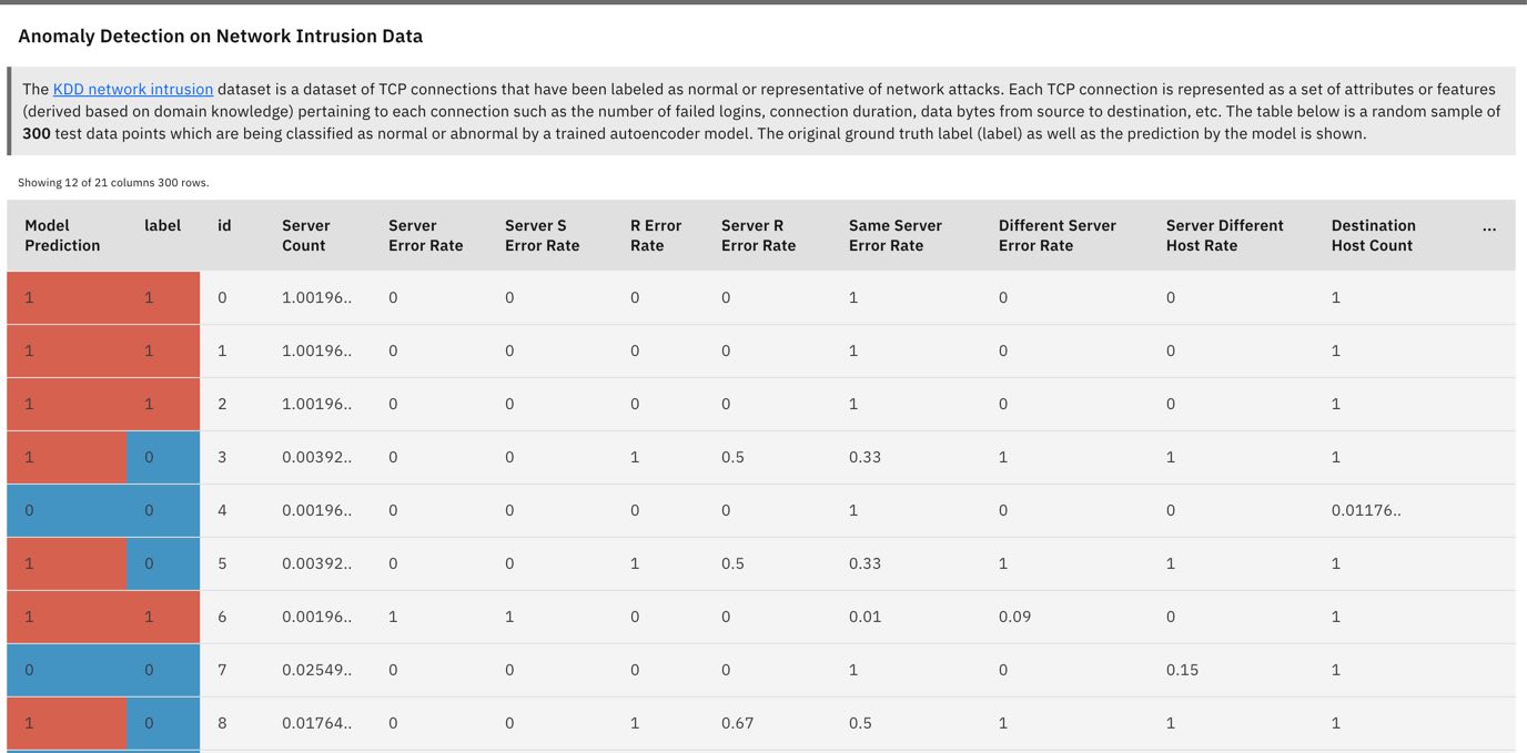
This repo contains experimental code used to implement deep learning techniques for the task of anomaly detection and launches an interactive dashboard to visualize model results applied to a network intrusion use case. We include implementations of several neural networks (Autoencoder, Variational Autoencoder, Bidirectional GAN, Sequence Models) in Tensorflow 2.0 and two other baselines (One Class SVM, PCA).
For an in-depth review of the concepts presented here, please consult the Cloudera Fast Forward report Deep Learning for Anomaly Detection. Additionally, two related prototypes are available for reference - Blip & Anomagram
| AutoEncoder | Variational AutoEncoder | BiGAN |
 |
 |
 |
| Seq2Seq | PCA | OCSVM |
 |
 |
 |
Anomalies - often referred to as outliers, abnormalities, rare events, or deviants - are data points or patterns in data that do not conform to a notion of normal behavior. Anomaly detection, then, is the task of finding those patterns in data that do not adhere to expected norms, given previous observations. The capability to recognize or detect anomalous behavior can provide highly useful insights across industries. Flagging unusual cases or enacting a planned response when they occur can save businesses time, costs, and customers. Hence, anomaly detection has found diverse applications in a variety of domains, including IT analytics, network intrusion analytics, medical diagnostics, financial fraud protection, manufacturing quality control, marketing and social media analytics, and more.
The underlying strategy for most approaches to anomaly detection is to first model normal behavior, and then exploit this knowledge to identify deviations (anomalies). In this repo, the process includes the following steps:
- Build a model of normal behavior using available data. Typically the model is trained on normal behavior data or assumes a small amount of abnormal data.
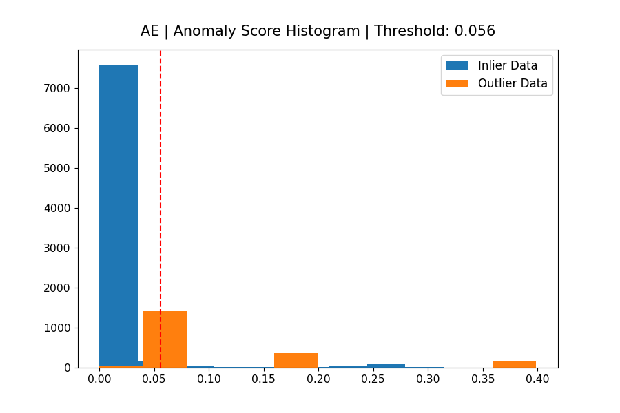
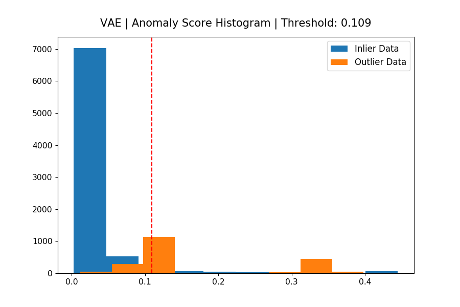
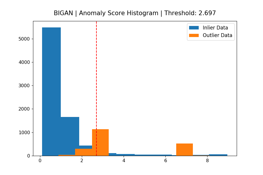
- Based on this model, assign an anomaly score to each data point that represents a measure of deviation from normal behavior. The models in this repo use a reconstruction error approach, where the model attempts to reconstruct a sample at test time, and uses the reconstruction error as an anomaly score. The intuition is that normal samples will be reconstructed with almost no error, while abnormal/unusual samples will be reconstructed with larger error margins.
- Apply a threshold on the anomaly score to determine which samples are anomalies.
As an illustrative example, an autoencoder model is trained on normal samples where the task is to reconstruct the input. At test time, we can use the reconstruction error (mean squared error) for each sample as anomaly scores.
├── data
│   ├── kdd
│   ├── kdd_data_gen.py
├── cml
│   ├── cml_build.py
│   ├── cml_servemodel.py
│   ├── install_deps.py
├── metrics
├── models
│   ├── ae.py
│   ├── bigan.py
│   ├── ocsvm.py
│   ├── pca.py
│   ├── seq2seq.py
│   ├── vae.py
├── utils
│   ├── data_utils.py
│   ├── eval_utils.py
│   ├── train_utils.py
├── train.py
├── test.pyThe data directory holds the KDD Network Intrusion dataset used the experiments and interactive dashboard. It contains a script (kdd_data_gen.py) that downloads the data, constructs train and test sets separated into inliers and outliers, and places those data files in the data/kdd directory.
The cml folder contains the artifacts needed to configure and launch the project on Cloudera Machine Learning (CML).
The models directory contains modules for each of the model implementations. Each module comes with code to specify parameters and methods for training and computing an anomaly score. It also serves as the holding location of saved models after training.
The utils directory holds helper functions that are referenced throughout different modules and scripts in the repo.
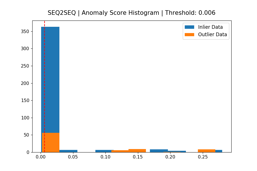
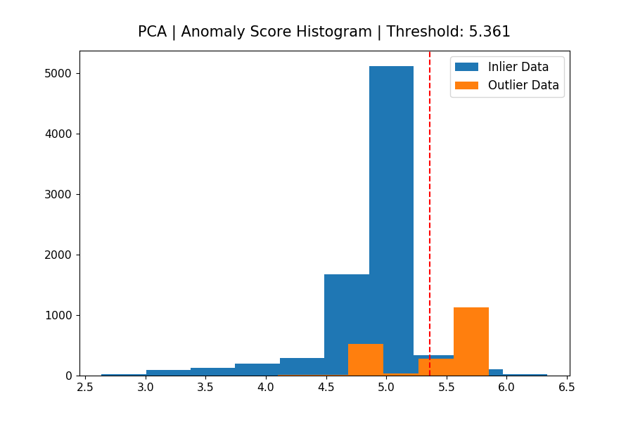
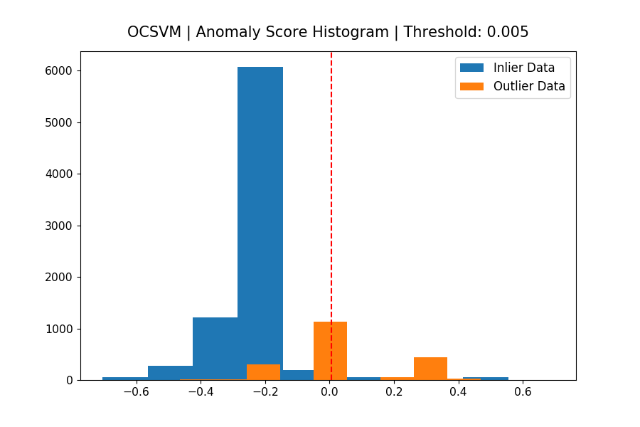
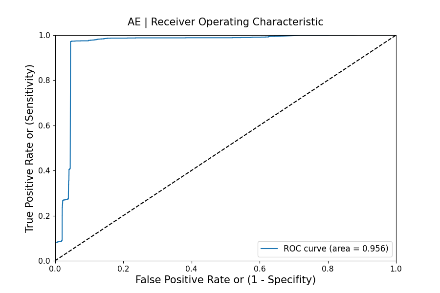
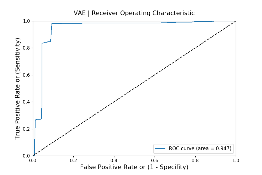
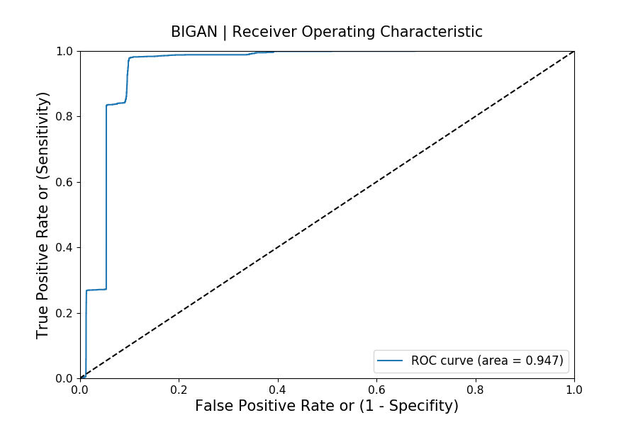
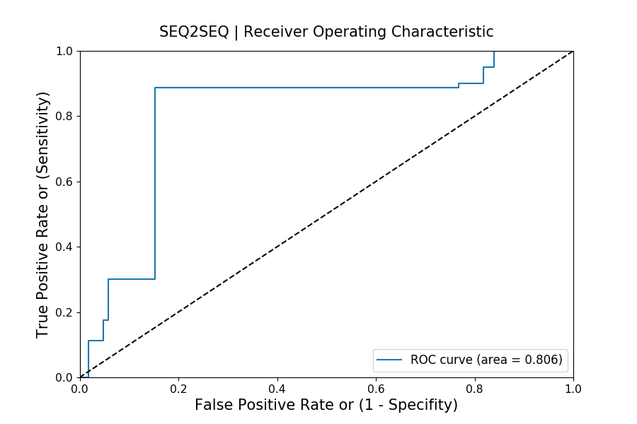
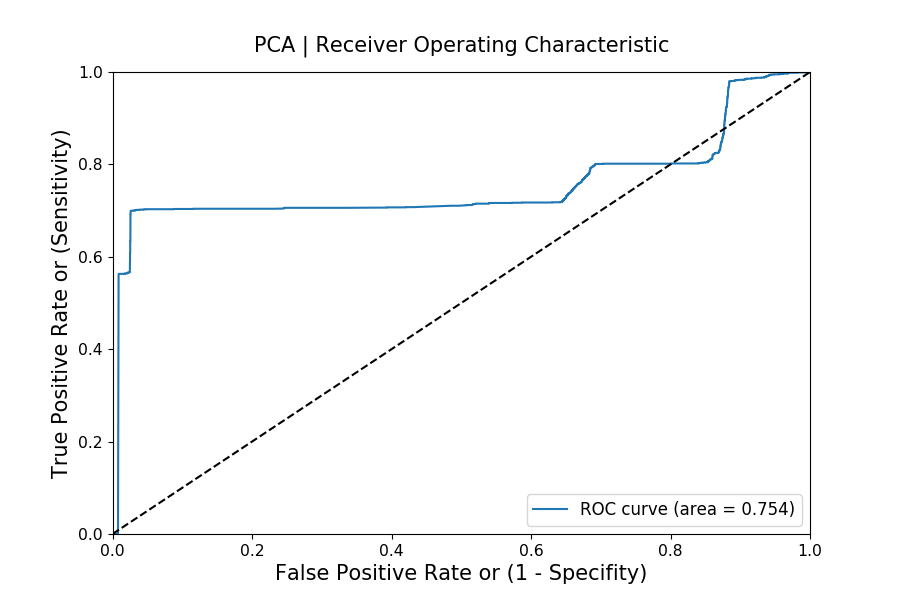
This script contains code to train and then evaluate each model by generating a histogram of anomaly scores assigned by each model, and ROC curve to assess model skill on the anomaly detection task. The general steps taken in the script are:
- Download the KDD dataset if not already downloaded
- Trains all of the models (Autoencoder, Variational Autoencoder, Bidirectional GAN, Sequence Models, PCA, OCSVM)
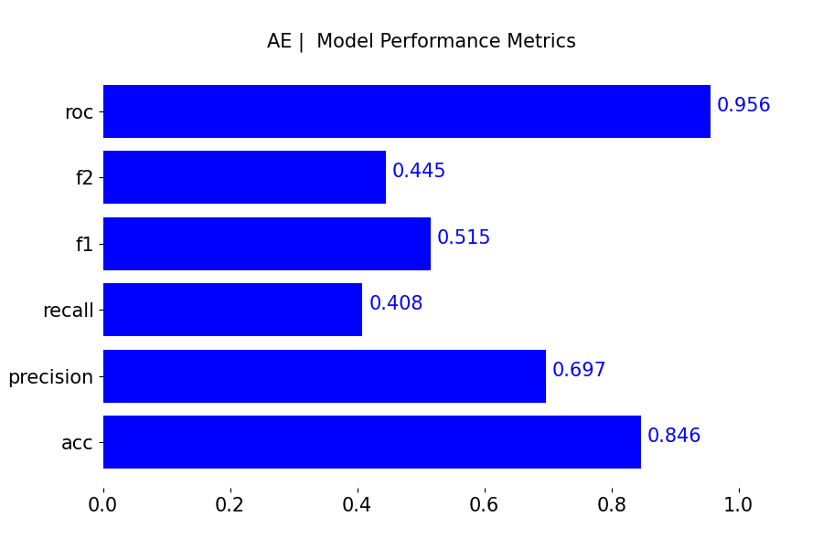
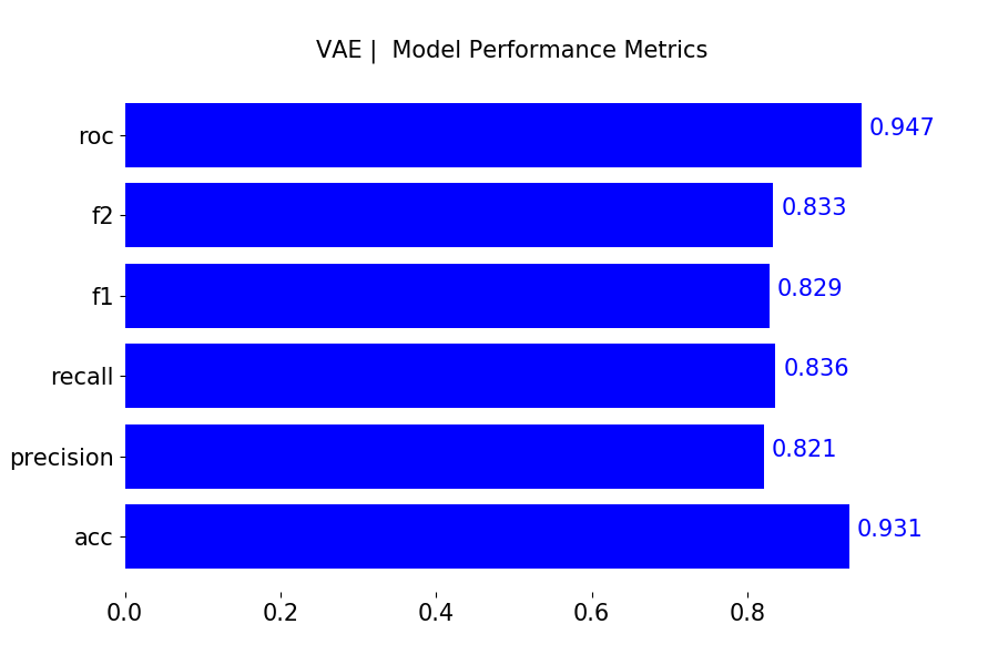
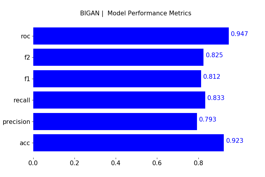
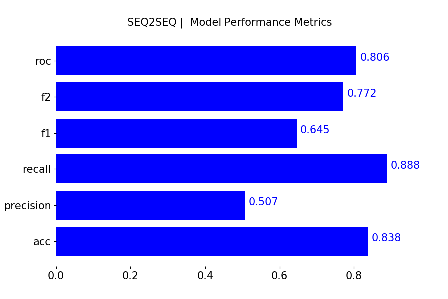
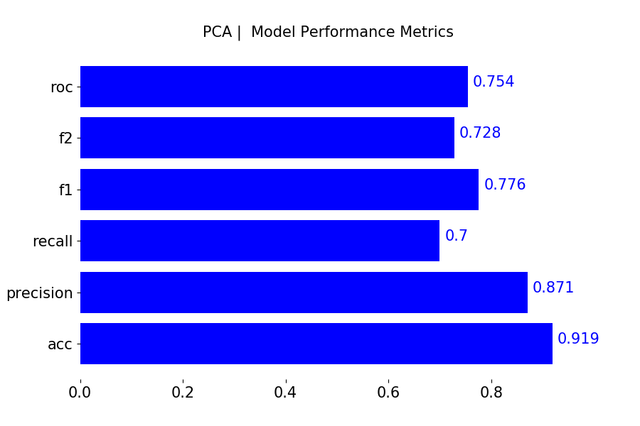
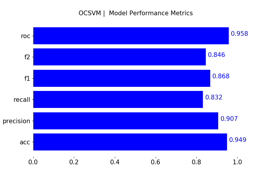
- Evaluates the models on a test split (8000 inliers, 2000 outliers). Generates charts on model performance: histogram of anomaly scores, ROC, general metrics (f1,f2, precision, recall, accuracy)
| AutoEncoder | Variational AutoEncoder | BiGAN |
 |
 |
 |
| Seq2Seq | PCA | OCSVM |
 |
 |
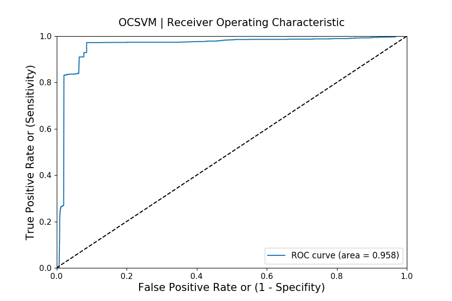 |
For each model, we use labeled test data to first select a threshold that yields the best accuracy and then report on metrics such as f1, f2, precision, and recall at that threshold. We also report on ROC (area under the curve) to evaluate the overall skill of each model. Given that the dataset we use is not extremely complex (18 features), we see that most models perform relatively well. Deep models (BiGAN, AE) are more robust (precision, recall, ROC AUC), compared to PCA and OCSVM. The sequence-to-sequence model is not particularly competitive, given the data is not temporal. On a more complex dataset (e.g., images), we expect to see (similar to existing research), more pronounced advantages in using a deep learning model.
For additional details on each model, see our report. Note that models implemented here are optimized for tabular data. For example, extending this to work with image data will usually require the use of convolutional layers (as opposed to dense layers) within the neural network models to achieve performant results.
| AutoEncoder | Variational AutoEncoder | BiGAN |
 |
 |
 |
| Seq2Seq | PCA | OCSVM |
 |
 |
 |
Given the differences between the deep learning methods discussed above (and their variants), it can be challenging to decide on the right model. When data contains sequences with temporal dependencies, a sequence-to-sequence model (or architectures with LSTM layers) can model these relationships well, yielding better results. For scenarios requiring principled estimates of uncertainty, generative models such as a VAE and GAN based approaches are suitable. For scenarios where the data is images, AEs, VAEs and GANs designed with convolution layers are suitable. The following table highlights the pros and cons of the different types of models, to provide guidance on when they are a good fit.
| Model | Pros | Cons |
|---|---|---|
| AutoEncoder |
|
|
| Variational AutoEncoder |
|
|
| GAN (BiGAN) |
|
|
| Sequence-to-Sequence Model |
|
|
| One Class SVM |
|
|
For users interested in deploying this application on Cloudera Machine Learning, there are three ways to launch the project:
- From Prototype Catalog - Navigate to the Prototype Catalog on a CML workspace, select the "Deep Learning for Anomaly Detection" tile, click "Launch as Project", click "Configure Project"
- As ML Prototype - In a CML workspace, click "New Project", add a Project Name, select "ML Prototype" as the Initial Setup option, copy in the repo URL, click "Create Project", click "Configure Project"
- Manual Setup - In a CML workspace, click "New Project", add a Project Name, select "Git" as the Initial Setup option. Launch a Python3 Workbench Session with at least 4GB of memory and run the
cml/cml_build.pyscript which will create a CML Application and provide a link to the UI.
Regardless of the launch method, the following steps are performed for you:
-
Install Dependencies - All necessary package dependencies are installed into the new project.
-
Model Training - A CML job is executed which consists of a call to
train.py. This in turn trains a model and saves the model to themodels/savedmodelfolder. -
Application Serving - A custom web application (shown above) makes requests to the model and visualizes results. To run the web application standalone run
python3 app/backend/app.py
