Overview

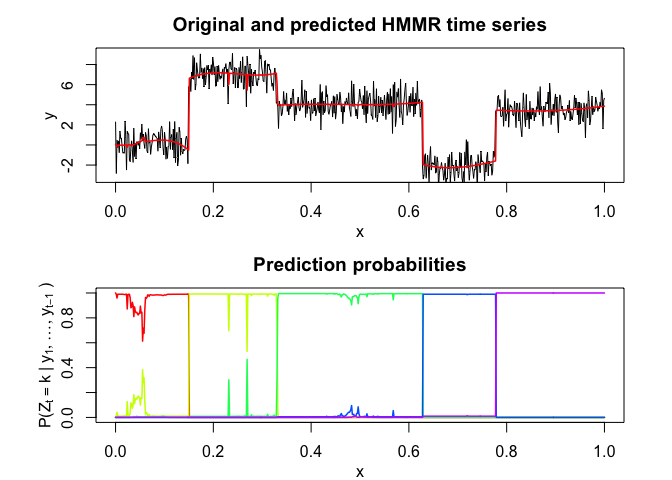
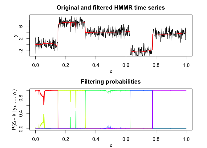
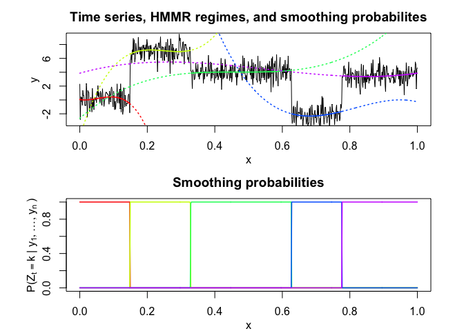
User-friendly and flexible algorithm for time series segmentation with a regression model governed by a hidden Markov process.

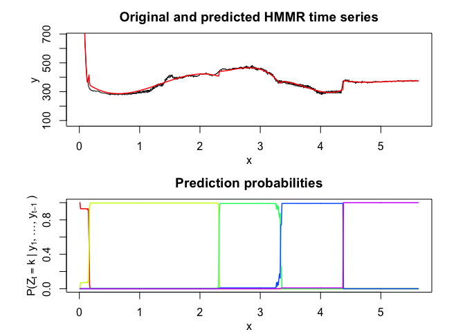
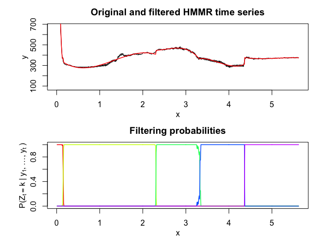
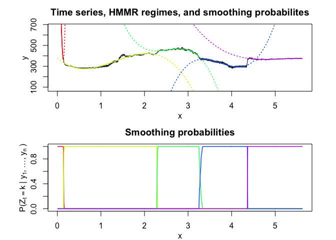
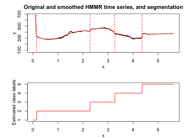
Hidden Markov Model Regression (HMMR) for segmentation of time series with regime changes. The model assumes that the time series is governed by a sequence of hidden discrete regimes/states, where each regime/state has Gaussian regressors as observations. The model parameters are estimated by MLE via the EM algorithm.

Installation

You can install the development version of HMMR from GitHub with:

# install.packages("devtools")
devtools::install_github("fchamroukhi/HMMR_r")

To build vignettes for examples of usage, type the command below instead:

# install.packages("devtools")
devtools::install_github("fchamroukhi/HMMR_r", 
                         build_opts = c("--no-resave-data", "--no-manual"), 
                         build_vignettes = TRUE)

Use the following command to display vignettes:

browseVignettes("HMMR")

Usage

library(HMMR)

# Application to a toy data set
data("toydataset")
x <- toydataset$x
y <- toydataset$y

K <- 5 # Number of regimes (states)
p <- 3 # Dimension of beta (order of the polynomial regressors)
variance_type <- "heteroskedastic" # "heteroskedastic" or "homoskedastic" model

n_tries <- 1
max_iter <- 1500
threshold <- 1e-6
verbose <- TRUE

hmmr <- emHMMR(X = x, Y = y, K, p, variance_type, n_tries, 
               max_iter, threshold, verbose)
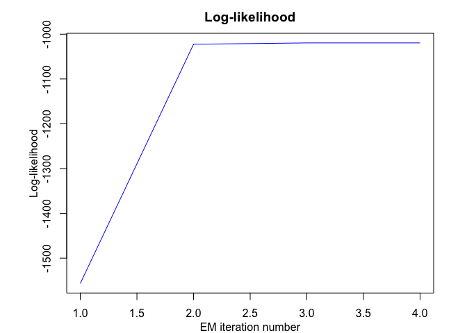
#> EM - HMMR: Iteration: 1 | log-likelihood: -1556.39696825601
#> EM - HMMR: Iteration: 2 | log-likelihood: -1022.47935723687
#> EM - HMMR: Iteration: 3 | log-likelihood: -1019.51830707432
#> EM - HMMR: Iteration: 4 | log-likelihood: -1019.51780361388

hmmr$summary()
#> ---------------------
#> Fitted HMMR model
#> ---------------------
#> 
#> HMMR model with K = 5 components:
#> 
#>  log-likelihood nu       AIC       BIC
#>       -1019.518 49 -1068.518 -1178.946
#> 
#> Clustering table (Number of observations in each regimes):
#> 
#>   1   2   3   4   5 
#> 100 120 200 100 150 
#> 
#> Regression coefficients:
#> 
#>       Beta(k = 1) Beta(k = 2) Beta(k = 3) Beta(k = 4) Beta(k = 5)
#> 1    6.031872e-02   -5.326689    -2.65064    120.8612    3.858683
#> X^1 -7.424715e+00  157.189455    43.13601   -474.9870   13.757279
#> X^2  2.931651e+02 -643.706204   -92.68115    598.3726  -34.384734
#> X^3 -1.823559e+03  855.171715    66.18499   -244.5175   20.632196
#> 
#> Variances:
#> 
#>  Sigma2(k = 1) Sigma2(k = 2) Sigma2(k = 3) Sigma2(k = 4) Sigma2(k = 5)
#>       1.220624      1.111487      1.080043     0.9779724      1.028399

hmmr$plot()

# Application to a real data set
data("realdataset")
x <- realdataset$x
y <- realdataset$y2

K <- 5 # Number of regimes (states)
p <- 3 # Dimension of beta (order of the polynomial regressors)
variance_type <- "heteroskedastic" # "heteroskedastic" or "homoskedastic" model

n_tries <- 1
max_iter <- 1500
threshold <- 1e-6
verbose <- TRUE

hmmr <- emHMMR(X = x, Y = y, K, p, variance_type, 
               n_tries, max_iter, threshold, verbose)
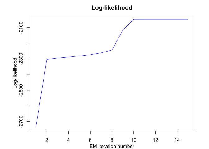
#> EM - HMMR: Iteration: 1 | log-likelihood: -2733.41028643114
#> EM - HMMR: Iteration: 2 | log-likelihood: -2303.24018378559
#> EM - HMMR: Iteration: 3 | log-likelihood: -2295.0470677529
#> EM - HMMR: Iteration: 4 | log-likelihood: -2288.57866215726
#> EM - HMMR: Iteration: 5 | log-likelihood: -2281.36756202518
#> EM - HMMR: Iteration: 6 | log-likelihood: -2273.50303676091
#> EM - HMMR: Iteration: 7 | log-likelihood: -2261.70334656117
#> EM - HMMR: Iteration: 8 | log-likelihood: -2243.43509121433
#> EM - HMMR: Iteration: 9 | log-likelihood: -2116.4610801575
#> EM - HMMR: Iteration: 10 | log-likelihood: -2046.73194777839
#> EM - HMMR: Iteration: 11 | log-likelihood: -2046.68328282973
#> EM - HMMR: Iteration: 12 | log-likelihood: -2046.67329222076
#> EM - HMMR: Iteration: 13 | log-likelihood: -2046.66915144265
#> EM - HMMR: Iteration: 14 | log-likelihood: -2046.66694236131
#> EM - HMMR: Iteration: 15 | log-likelihood: -2046.66563379017

hmmr$summary()
#> ---------------------
#> Fitted HMMR model
#> ---------------------
#> 
#> HMMR model with K = 5 components:
#> 
#>  log-likelihood nu       AIC       BIC
#>       -2046.666 49 -2095.666 -2201.787
#> 
#> Clustering table (Number of observations in each regimes):
#> 
#>   1   2   3   4   5 
#>  14 214  99 109 126 
#> 
#> Regression coefficients:
#> 
#>     Beta(k = 1) Beta(k = 2) Beta(k = 3) Beta(k = 4) Beta(k = 5)
#> 1       2152.64   379.75158   5211.1759 -14306.4654  6417.62823
#> X^1   -12358.67  -373.37266  -5744.7879  11987.6666 -3571.94086
#> X^2  -103908.33   394.49359   2288.9418  -3233.8021   699.55894
#> X^3   722173.26   -98.60485   -300.7686    287.4567   -45.42922
#> 
#> Variances:
#> 
#>  Sigma2(k = 1) Sigma2(k = 2) Sigma2(k = 3) Sigma2(k = 4) Sigma2(k = 5)
#>       9828.793      125.3346      58.71053      105.8328      15.66317

hmmr$plot()

Model selection

In this package, it is possible to select models based on information criteria such as BIC, AIC and ICL.

The selection can be done for the two following parameters:

K: The number of regimes;
p: The order of the polynomial regression.

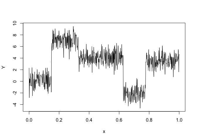
Let’s select a HMMR model for the following time series Y:

data("toydataset")
x <- toydataset$x
y <- toydataset$y

plot(x, y, type = "l", xlab = "x", ylab = "Y")

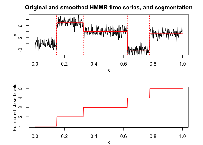
selectedhmmr <- selectHMMR(X = x, Y = y, Kmin = 2, Kmax = 6, pmin = 0, pmax = 3)
#> The HMMR model selected via the "BIC" has K = 5 regimes 
#>  and the order of the polynomial regression is p = 0.
#> BIC = -1136.39152222095
#> AIC = -1059.76780111041

selectedhmmr$plot(what = "smoothed")