Link to my jupyter notebook containing my code
Build a Traffic Sign Recognition Project
The goals / steps of this project are the following:
- Load the data set (see below for links to the project data set)
- Explore, summarize and visualize the data set
- Design, train and test a model architecture
- Use the model to make predictions on new images
- Analyze the softmax probabilities of the new images
- Summarize the results with a written report
Here I will consider the rubric points individually and describe how I addressed each point in my implementation.
1. Provide a Writeup / README that includes all the rubric points and how you addressed each one. You can submit your writeup as markdown or pdf. You can use this template as a guide for writing the report. The submission includes the project code.
This document!
1. Provide a basic summary of the data set. In the code, the analysis should be done using python, numpy and/or pandas methods rather than hardcoding results manually.
I used the pandas library to calculate summary statistics of the traffic signs data set:
- The size of training set is 34799
- The size of the validation set is 4410
- The size of test set is 12630
- The shape of a traffic sign image is (height: 32 width: 32 channel: 3)
- The number of unique classes/labels in the data set is 43
- Color values go from 0 to 255
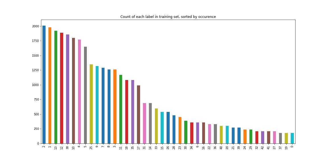
Here is an exploratory visualization of the data set. It is a bar chart showing how the number of occurences of each traffic sign for the training set.
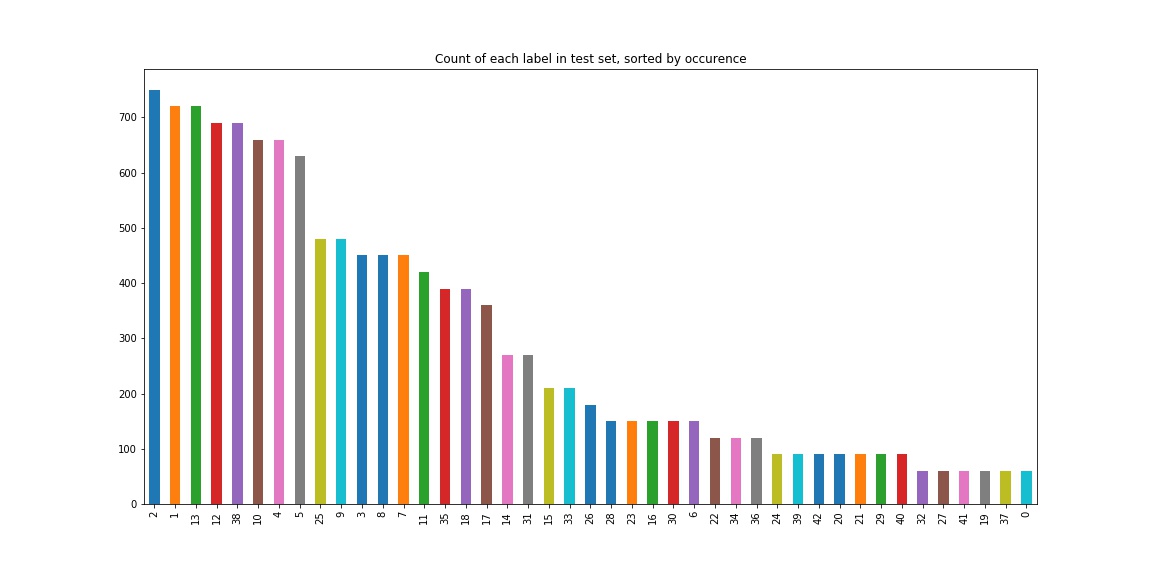
For the test set looks like this:
Each traffic sign has a similar occurence in both sets but there is a significant difference in the total occurence between the traffic signs. This might lead to a bias of some sign as they are more often in the set.
1. Describe how you preprocessed the image data. What techniques were chosen and why did you choose these techniques? Consider including images showing the output of each preprocessing technique. Pre-processing refers to techniques such as converting to grayscale, normalization, etc.
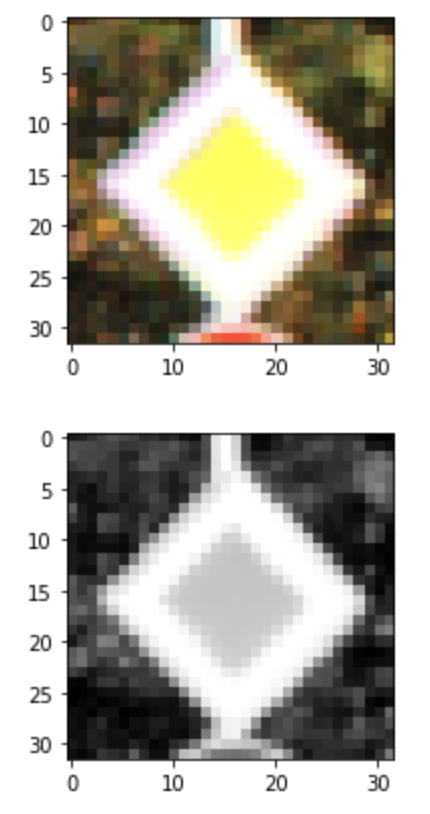
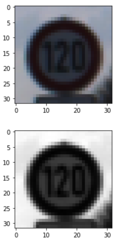
As a first step, I decided to convert the images to grayscale because my accuracy was significantly better when using it. The input is thereby simplified and smaller by a factor of 3.
Here are two examples of a traffic sign images before and after grayscaling.
As a last step, I normalized the image data because this makes the model a lot faster and easier to train. I mapped the original value range of (0 to 255) to a range from -1.0 to 1.0 .
2. Describe what your final model architecture looks like including model type, layers, layer sizes, connectivity, etc.) Consider including a diagram and/or table describing the final model.
My final model consisted of the following layers:
| Layer | Description |
|---|---|
| Input | 32x32x3 RGB image |
| Convolution 5x5 | 1x1 stride, valid padding, outputs 32x32x64 |
| RELU | |
| Max pooling | 2x2 stride, outputs 16x16x64 |
| Convolution 5x5 | 1x1 stride, valid padding, outputs 32x32x64 |
| RELU | |
| Convolution 5x5 | 1x1 stride, valid padding, outputs 32x32x64 |
| RELU | |
| Max pooling | 2x2 stride, outputs 16x16x64 |
| Flatten | flattening to output of 576 |
| Fully connected | output 120 |
| Dropout | keep rate 0.7 |
| Fully connected | output 84 |
| Dropout | keep rate 0.7 |
| Fully connected | output 43 (different traffic signs) |
3. Describe how you trained your model. The discussion can include the type of optimizer, the batch size, number of epochs and any hyperparameters such as learning rate.
| Parameters | Values |
|---|---|
| learning rate | 0.0025 |
| epochs | 15 |
| batch size | 128 |
| optimizer | Adam optimizer |
| loss function | Cross entropy loss |
| training operation | minimze loss function |
My model is trained with the adam optimizer trying to minimze the cross entropy loss as we desire a classification of the image.
I played a lot with the parameters, especially epochs and the learning rate. If I increase the learning rate I can't optimize it precise enough on the other hand if i decrease the learning rate it takes to many epochs to complete and it gets stuck in local minima.
More epochs or a larger batch size don't improve my result.
4. Describe the approach taken for finding a solution and getting the validation set accuracy to be at least 0.93. Include in the discussion the results on the training, validation and test sets and where in the code these were calculated. Your approach may have been an iterative process, in which case, outline the steps you took to get to the final solution and why you chose those steps. Perhaps your solution involved an already well known implementation or architecture. In this case, discuss why you think the architecture is suitable for the current problem.
My final model results were:
- training set accuracy of 99.8%
- validation set accuracy of 97.43%
- test set accuracy of 95.3%
If an iterative approach was chosen:
I choose the LeNet architecture as recommended. I started out be feeding the colored into the model. The model had to be adapted to accept colored images.
This paper only used the greyscaled image so I tried that out and my model jumped accuracy immediatly.
I added another convolution layer and increased the number of filters of the exisiting convolution layers to capture the added complexity of the traffic sign compared to the character recognition, which were presented in the course with this model. As a result the output length of the flatten layer increased.
After I noticed some overfitting I added a dropout layer between the fully connected layers, respectively. This improved the validation accuracy.
By adjusting the hyperparameter I passed the minimum accuracy of 93%. I increased the learning rate from 0.001 to 0.0025 and the epochs from 10 to 15.
1. Choose five German traffic signs found on the web and provide them in the report. For each image, discuss what quality or qualities might be difficult to classify.
Here are five German traffic signs that I found on the web:
The first image might be difficult to classify because it is occluded by another image. The second image might be difficult to classify because it is occluded by another sign in the background. The thrid image should be easy to classify. The fourth image might be difficult to classify because there is snow on the sign which makes it harder to read. The fifth image might be difficult to classify because there is snow on the sign which makes it harder to read.
2. Discuss the model's predictions on these new traffic signs and compare the results to predicting on the test set. At a minimum, discuss what the predictions were, the accuracy on these new predictions, and compare the accuracy to the accuracy on the test set (OPTIONAL: Discuss the results in more detail as described in the "Stand Out Suggestions" part of the rubric).
Here are the results of the prediction:
| Image | Prediction |
|---|---|
| Traffic signals | Road work |
| Bicycles crossing | Children crossing |
| Right-of-way at the next intersection | Right-of-way at the next intersection |
| General caution | Traffic signals |
| Slippery Road | Slippery Road |
The model was able to correctly guess 4 of the 5 traffic signs, which gives an accuracy of 80%. This compares favorably to the accuracy on the test set of ...
3. Describe how certain the model is when predicting on each of the five new images by looking at the softmax probabilities for each prediction. Provide the top 5 softmax probabilities for each image along with the sign type of each probability.
The code for making predictions on my final model is located in the 15th cell of the jupyter notebook.
I have deliberately chosen images that are hard to predict. :)
For the first image, the model is relatively sure that this is a roads work sign (probability of 0.6), and is acctually a traffic signals sign which is occluded by a Bicycles crossing sign. Both are in the top 5 and traffic signal even on position number 2
The top five soft max probabilities were
| Probability | Prediction |
|---|---|
| .62 | Road work |
| .25 | Traffic signals |
| .10 | General caution |
| .01 | Bicycles crossing |
| .006 | Road narrows on the right |
For the second image is unsure that it is children crossing (probability of 0.48) and it is wrong as it is bicycles crossing. This sign has a probability of 0.04 but it is still in the top 5.
The top five soft max probabilities were
| Probability | Prediction |
|---|---|
| .48 | Children crossing |
| .21 | Dangerous curve to the right |
| .07 | Bumpy road |
| .04 | Bicycles crossing |
| .04 | Speed limit (120km/h) |
For the third image it is absolutly sure that it is a Right-of-way at the next intersection and it is correct. It shows that the model has confidence for easy images.
The top five soft max probabilities were
| Probability | Prediction |
|---|---|
| .99 | Right-of-way at the next intersection |
| .00004 | Beware of ice/snow |
| .000004 | Double curve |
| .000004 | Priority road |
| .000001 | Pedestrians |
For the fourth image it is unsure that it is a no passing sign but it is a no passing sign. It has a similar probability as the sign in the second position which is also a round sign (speed limit).
The top five soft max probabilities were
| Probability | Prediction |
|---|---|
| .26 | No passing |
| .23 | Speed limit (120km/h) |
| .07 | Traffic signals |
| .05 | Roundabout mandatory |
| .04 | Dangerous curve to the right |
For the fifth image is pretty sure that it is traffic signals but the model is wrong since it is a general caution sign, which the model predicted second with a very low probability of 0.03.
The top five soft max probabilities were
| Probability | Prediction |
|---|---|
| .75 | Traffic signals |
| .03 | General caution |
| .006 | Bumpy road |
| .001 | Dangerous curve to the right |
| .001 | Speed limit (120km/h) |


