Knitron brings the power of IPython and matplotlib to knitr.
It also brings workspace-like interaction for Python to knitr, so you can define a variable in one chunk
x = 5and access it in a following chunk
x + 1## 6
- R with knitr and devtools
- A recent version of IPython (knitron relies on the new
IPython.parallelAPI) - pyzmq
These can be installed by executing (in a shell):
Rscript -e "install.packages('knitr')"
apt-get install python-dev libzmq3-dev libgit2-dev # on Debian and derivates
Rscript -e "install.packages('devtools')"
pip install IPython
pip install pyzmq
In even newer version of IPython, the parallel API has been split in a
separate package, usually called ipyparallel:
pip install ipyparallelIn R:
library(devtools)
install_github("knitron", "fhirschmann")In order to provide a persistent state for multiple chunks in a document, knitron makes use of IPython's architecture for parallel computing. An IPython cluster is started into the background before the chunks are being processed.
library(knitron)That's it! Now you can use IPython in knitr using the engine = 'ipython' option
(see the source code
of this page for an example).
By default, the knitr IPython profile will be used. You can change this using the knitron.profile chunk option. If the profile doesn't exist already, it will be created and can then be modified (take a look at ~/.ipython/profile_knitr). When the first chunk for each profile gets evaluated, a cluster with one engine will be spawned by knitron if it isn't already running. You can also spawn your cluster in a parallel process using
ipcluster start --profile=knitr --n=1
If the cluster has been spawned by knitron, it will be terminated on exit.
To use knitron in RStudio, the knitron library needs to be loaded in an R chunk. This can usually be done in the preamble, i.e. for LaTeX before executing any IPython chunk, define:
<<setup, echo = F>>=
library(knitron)
@
An exemplary document showing the use of knitron inside RStudio is available.
Knitron imports matplotlib and pyplot (as plt) unless knitron.matplotlib is set
to FALSE. For figures to appear after the chunk, pyplot is expected to be used.
The following knitron-specific chunk options are available in knitron:
knitron.profile = "knitr"specifies the IPython profile to be used for the evaluation of the chunk.knitron.matplotlib = TRUEloads matplotlib and pyplot (asplt) before executing a chunk.knitron.print = "auto"will print the string representation of the last object in a code chunk. By default, it will not print the string representation of a plot. Other values for this option areTRUEandFALSE.
Most of the original knitr chunk options are supported, including
fig.pathfig.widthandfig.heightdpidev'pdf' for LaTeX and 'png' for HTML/markdown; most of the other devices (e.g. svg, Cairo_png) are supported too
However, there are limitations to some options:
fig.showonly supportshold, i.e. all figures are placed at the end of each code chunkdevcurrently supports only one device per chunk, i.e. you cannot give a character vector so that two plots with different devices are generated
IPython's magic functions are supported too, of course. But there are
some limitations, i.e. magic functions that insert text into the IPython
shell like %load without executing them don't work. Likewise, magics
that are meant for interactive use like %man and %edit cannot work in
knitr.
from time import sleep

%time sleep(0.5)
## CPU times: user 0 ns, sys: 0 ns, total: 0 ns
## Wall time: 500 ms
%whos## Variable Type Data/Info
## ----------------------------------------------------
## f function <function f at 0x7f504addf140>
## matplotlib module <module 'matplotlib' from<...>matplotlib/__init__.pyc'>
## np module <module 'numpy' from '/us<...>ages/numpy/__init__.pyc'>
## plt module <module 'matplotlib.pyplo<...>s/matplotlib/pyplot.pyc'>
## sleep builtin_function_or_method <built-in function sleep>
## t1 ndarray 50: 50 elems, type `float64`, 400 bytes
## t2 ndarray 250: 250 elems, type `float64`, 2000 bytes
## x int 5
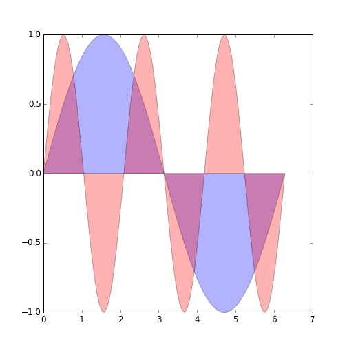
import numpy as np
x = np.linspace(0, 2 * np.pi, 100)
y1 = np.sin(x)
y2 = np.sin(3 * x)
plt.fill(x, y1, 'b', x, y2, 'r', alpha=0.3)
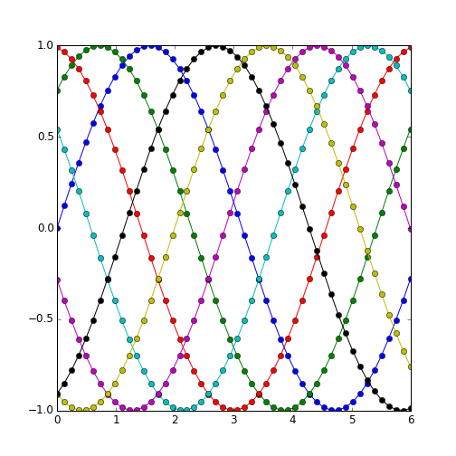
L = 6
x = np.linspace(0, L)
ncolors = len(plt.rcParams['axes.color_cycle'])
shift = np.linspace(0, L, ncolors, endpoint=False)
for s in shift:
plt.plot(x, np.sin(x + s), 'o-')## /usr/lib/python2.7/dist-packages/matplotlib/__init__.py:894: UserWarning: axes.color_cycle is deprecated and replaced with axes.prop_cycle; please use the latter.
## warnings.warn(self.msg_depr % (key, alt_key))


