In this work we will use data mining techniques on collected wine sets and evaluate wine quality by given raw data.
Wine can be classified by human experts or by physicochemical laboratory tests – pH or alcohol values or density determination.
But there is another method how to classify wine.
Input variables (based on physicochemical tests):
1 - fixed acidity
2 - volatile acidity
3 - citric acid
4 - residual sugar
5 - chlorides
6 - free sulfur dioxide
7 - total sulfur dioxide
8 - density
9 - pH
10 - sulphates
11 - alcohol
Output variable (based on sensory data):
12 - quality (score between 0 and 10)
from sklearn.cross_validation import train_test_split
from sklearn.linear_model import LinearRegression
from sklearn.metrics import mean_squared_error
from sklearn.ensemble import RandomForestRegressor

import numpy as np
import pandas as pd
import statsmodels.stats.api as sm

%pylab inline
Populating the interactive namespace from numpy and matplotlib
# Read data
wine = pd.read_csv('wine_data.csv', sep='\t')wine.head()| Type | Fixed acidity (g/l) | Volatile acidity (g/l) | Citric acid (g/l) | Residual sugar (g/l) | Chlorides (g/l) | Free sulfur dioxide (mg/l) | Total sulfur dioxide (mg/l) | Density (g/cm3) | pH | Sulphates (g/l) | Alcohol (%) | quality | |
|---|---|---|---|---|---|---|---|---|---|---|---|---|---|
| 0 | red | 7.4 | 0.70 | 0.00 | 1.9 | 0.076 | 11 | 34 | 0.9978 | 3.51 | 0.56 | 9.4 | 5 |
| 1 | red | 7.8 | 0.88 | 0.00 | 2.6 | 0.098 | 25 | 67 | 0.9968 | 3.20 | 0.68 | 9.8 | 5 |
| 2 | red | 7.8 | 0.76 | 0.04 | 2.3 | 0.092 | 15 | 54 | 0.9970 | 3.26 | 0.65 | 9.8 | 5 |
| 3 | red | 11.2 | 0.28 | 0.56 | 1.9 | 0.075 | 17 | 60 | 0.9980 | 3.16 | 0.58 | 9.8 | 6 |
| 4 | red | 7.4 | 0.70 | 0.00 | 1.9 | 0.076 | 11 | 34 | 0.9978 | 3.51 | 0.56 | 9.4 | 5 |
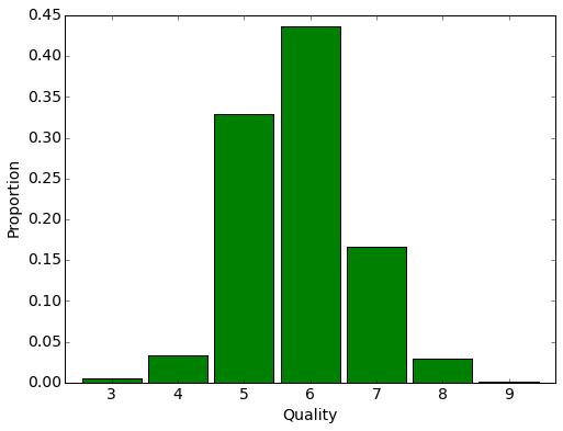
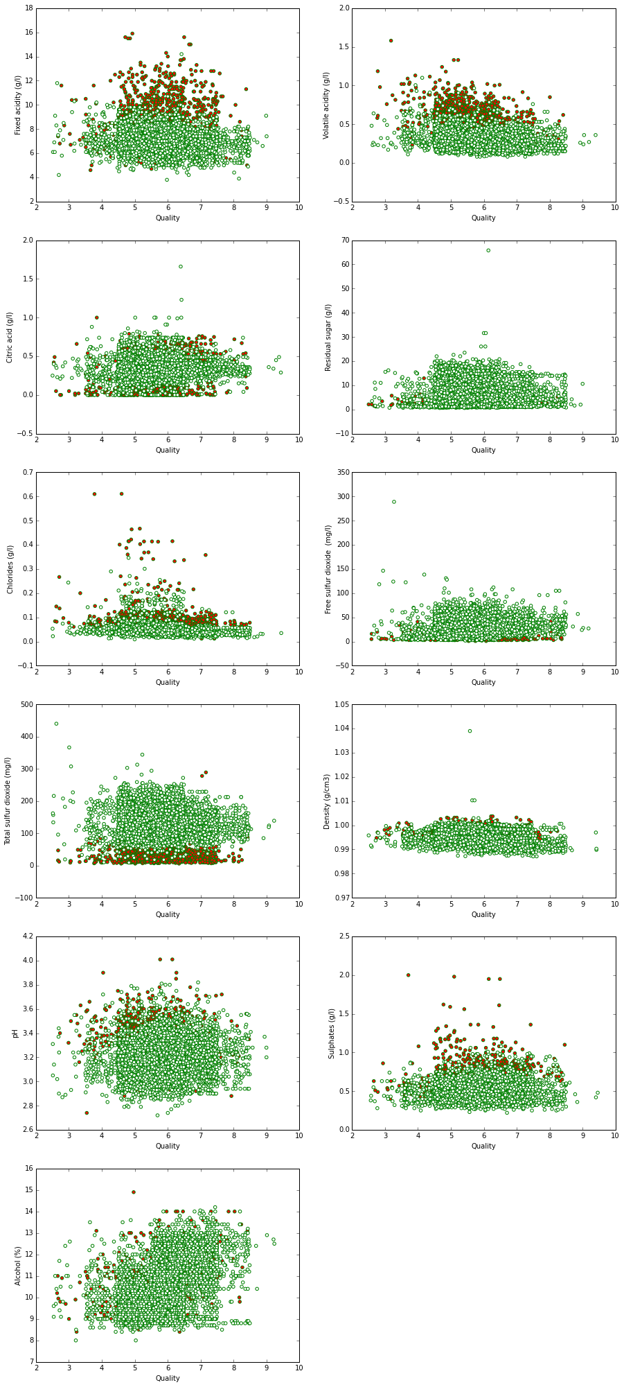
We see 11 signs describing the chemical composition of the wines. Here is the distribution of expert evaluation of wines in the sample:
plt.figure(figsize(8,6))
stat = wine.groupby('quality')['quality'].agg(lambda x : float(len(x))/wine.shape[0])
stat.plot(kind='bar', fontsize=14, width=0.9, color="green")
plt.xticks(rotation=0)
plt.ylabel('Proportion', fontsize=14)
plt.xlabel('Quality', fontsize=14)
<matplotlib.text.Text at 0x7f20f8773350>
y = wine[['Type', 'quality']]
y.head()| Type | quality | |
|---|---|---|
| 0 | red | 5 |
| 1 | red | 5 |
| 2 | red | 5 |
| 3 | red | 6 |
| 4 | red | 5 |
wine.groupby('Type')['Type'].count()Type
red 1599
white 4898
Name: Type, dtype: int64
We separate 25% of the set for the quality prediction control.
from sklearn.cross_validation import train_test_split

X_train, X_test, y_train, y_test = train_test_split(wine.ix[:, wine.columns != 'quality'],
                                                    wine['quality'],
test_size=0.25)X_train['Type'] = X_train['Type'].apply(lambda x : -1 if x == 'red' else 1)
X_test['Type'] = X_test['Type'].apply(lambda x : -1 if x == 'red' else 1)If we do not have any more information about the wines, our best guess on the assessment – - the average, available in the training set:
np.mean(y_train)5.8169129720853858
If we predict this value assessment of all the winse oin the training set, we get the average square error.
sqrt(mean_squared_error([np.mean(y_train)]*len(y_train), y_train))0.87670621485856171
and on the test
sqrt(mean_squared_error([np.mean(y_train)]*len(y_test), y_test))0.8625590794770277
On the test sample the error is greater, since we evaluate the average by the teaching. This is a natural effect. To clarify our prediction, it is possible to predict the value of every wine by the average estimation of wines of the same type in the sample:
regressor = LinearRegression()
regressor.fit(X_train['Type'].reshape(-1,1), y_train)
LinearRegression(copy_X=True, fit_intercept=True, n_jobs=1, normalize=False)
y_train_predictions = regressor.predict(X_train['Type'].reshape(-1,1))y_test_predictions = regressor.predict(X_test['Type'].reshape(-1,1))Prediction errors have decreased slightly:
sqrt(mean_squared_error(y_train_predictions, y_train))0.87064224152662018
sqrt(mean_squared_error(y_test_predictions, y_test))0.85579069866207058
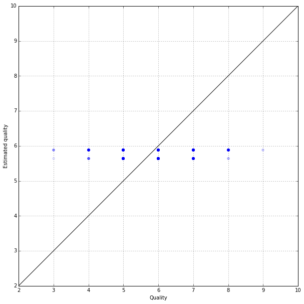
Here is the true evaluation of wines and their average prediction by the types on a test sample:
pyplot.figure(figsize(10,10))
pyplot.scatter(y_test, y_test_predictions, color="blue", alpha=0.1)
pyplot.xlim(2,10)
pyplot.ylim(2,10)
plot(range(11), color='black')
grid()
plt.xlabel('Quality')
plt.ylabel('Estimated quality')
<matplotlib.text.Text at 0x7f20dd856f10>
def fun(v):
    return v + np.random.uniform(low=-0.5,
                                 high=0.5,
                                 size=len(v))

pyplot.figure(figsize(15, 35))
for i in range (1, 12):
    pyplot.subplot(6, 2, i)
    pyplot.scatter(fun(wine['quality']), wine.ix[:, i],
                   color=wine["Type"],
                   edgecolors="green")
    pyplot.xlabel('Quality')
pyplot.ylabel(str(wine.columns[i]))To begin with, let us construct the linear regression model.
lm = LinearRegression()
lm.fit(X_train, y_train)
LinearRegression(copy_X=True, fit_intercept=True, n_jobs=1, normalize=False)
The prediction errors were essentially reduced:
sqrt(mean_squared_error(lm.predict(X_train), y_train))0.73840949206442807
sqrt(mean_squared_error(lm.predict(X_test), y_test))0.71457788648123488
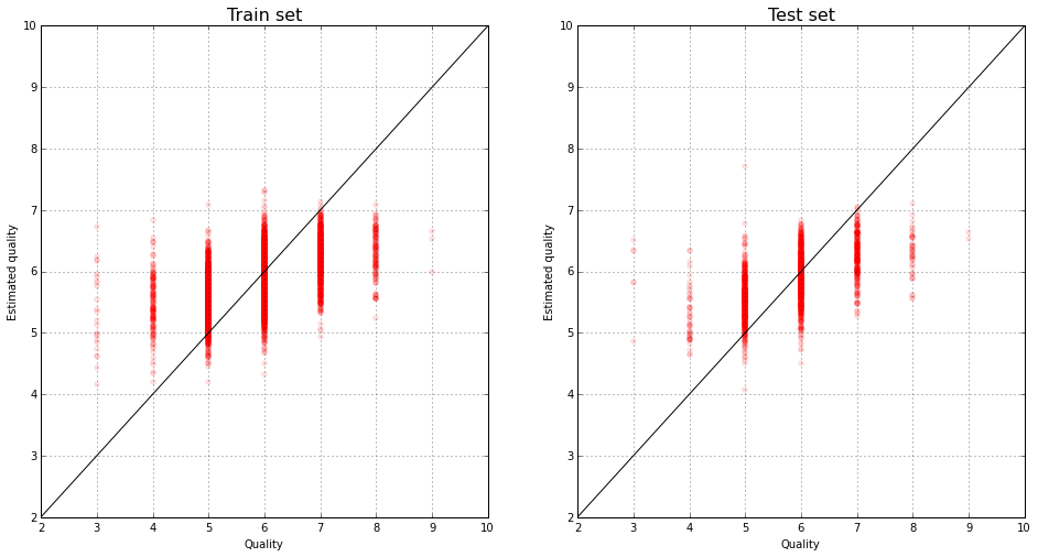
The true evaluation of wines and their predictions by the linear model:
plt.figure(figsize(16,8))
plt.subplot(121)
pyplot.scatter(y_train, lm.predict(X_train), color="red", alpha=0.1)
pyplot.xlim(2,10)
pyplot.ylim(2,10)
plot(range(11), color='black')
grid()
pyplot.title('Train set', fontsize=16)
pyplot.xlabel('Quality')
pyplot.ylabel('Estimated quality')

plt.subplot(122)
pyplot.scatter(y_test, lm.predict(X_test), color="red", alpha=0.1)
pyplot.xlim(2,10)
pyplot.ylim(2,10)
plot(range(11), color='black')
grid()
pyplot.title('Test set', fontsize=16)
pyplot.xlabel('Quality')
pyplot.ylabel('Estimated quality')
<matplotlib.text.Text at 0x7f2087f41190>
We calculate the coefficient of determination - the proportion by the explained model of the disperse response.
lm.score(X_test, y_test)0.31365659929719758
We construct the random forest on the teaching set:
rf = RandomForestRegressor(n_estimators=100, min_samples_leaf=3)rf.fit(X_train, y_train)RandomForestRegressor(bootstrap=True, criterion='mse', max_depth=None,
max_features='auto', max_leaf_nodes=None, min_samples_leaf=3,
min_samples_split=2, min_weight_fraction_leaf=0.0,
n_estimators=100, n_jobs=1, oob_score=False, random_state=None,
verbose=0, warm_start=False)
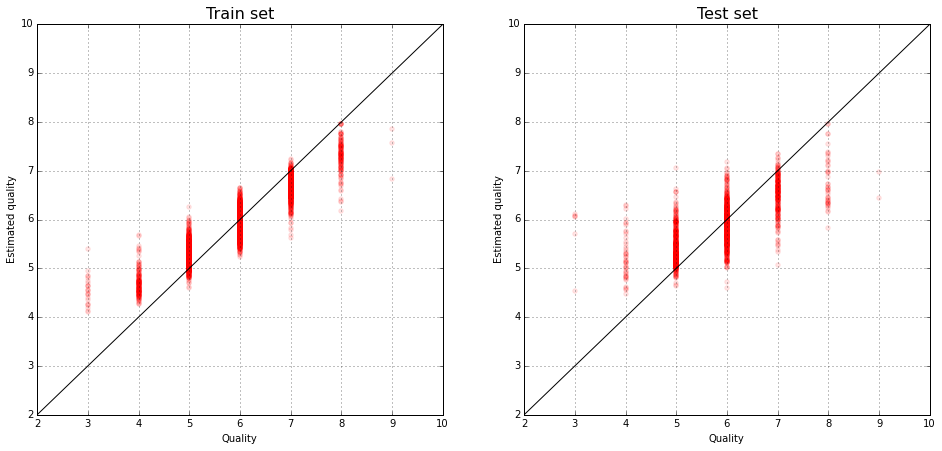
The quality has increased, though the model has been retrained.
sqrt(mean_squared_error(rf.predict(X_train), y_train))0.35262460471153395
sqrt(mean_squared_error(rf.predict(X_test), y_test))0.60694168473930055
The true evaluation of wines and their predictions by the random forest:
plt.figure(figsize(16,7))
plt.subplot(121)
pyplot.scatter(y_train, rf.predict(X_train), color="red", alpha=0.1)
pyplot.xlim(2,10)
pyplot.ylim(2,10)
plot(range(11), color='black')
grid()
pyplot.title('Train set', fontsize=16)
pyplot.xlabel('Quality')
pyplot.ylabel('Estimated quality')

plt.subplot(122)
pyplot.scatter(y_test, rf.predict(X_test), color="red", alpha=0.1)
pyplot.xlim(2,10)
pyplot.ylim(2,10)
plot(range(11), color='black')
grid()
pyplot.title('Test set', fontsize=16)
pyplot.xlabel('Quality')
pyplot.ylabel('Estimated quality')
<matplotlib.text.Text at 0x7f20878b3ad0>
The coefficient of determination for the random forest:
rf.score(X_test, y_test)0.50485060884990918
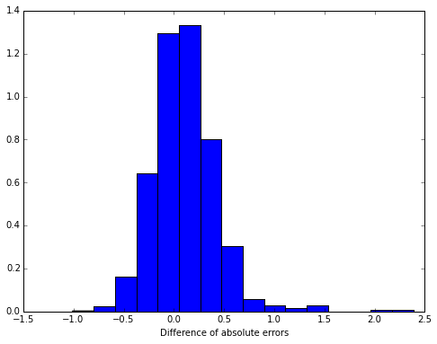
We compare the errors of the linear regression and random forest on a test sample:
plt.figure(figsize(8,6))
plt.hist(abs(y_test - lm.predict(X_test)) - abs(y_test - rf.predict(X_test)), bins=16, normed=True)
plt.xlabel('Difference of absolute errors')
<matplotlib.text.Text at 0x7f208792e510>
The differences between the average absolute errors are significant:
tmeans = sm.CompareMeans(sm.DescrStatsW(abs(y_test - lm.predict(X_test))),
                         sm.DescrStatsW(abs(y_test - rf.predict(X_test))))

tmeans.ttest_ind(alternative='two-sided', usevar='pooled', value=0)[1]
6.0766386407976045e-13
95% confidence interval for the average difference of absolute errors.
tmeans.tconfint_diff(alpha=0.05, alternative='two-sided', usevar='pooled')(0.079701943166600675, 0.13903686377836694)
That is, using our random forest instead of linear regression, we predict the expert evaluation more accurately. Let’s see what signs have the greatest predictive power:
importances = pd.DataFrame(zip(X_train.columns, rf.feature_importances_))
importances.columns = ['feature name', 'importance']
importances.sort(ascending=False)
The alcohol content has the greatest influence on the expert evaluation of wine quality.
In this work we solved the regression problem. The algorithms we chose are called linear regression and random forest. We predict that random forest has a better value. It is more exact. The alcohol content has the greatest influence on the expert evaluation of wine quality. The prediction model in this work can bear quite good results.
Citation Request: This dataset is public available for research. The details are described in [Cortez et al., 2009]. Please include this citation if you plan to use this database:
P. Cortez, A. Cerdeira, F. Almeida, T. Matos and J. Reis. Modeling wine preferences by data mining from physicochemical properties. In Decision Support Systems, Elsevier, 47(4):547-553. ISSN: 0167-9236.
Available at: [@Elsevier] http://dx.doi.org/10.1016/j.dss.2009.05.016 [bib] http://www3.dsi.uminho.pt/pcortez/dss09.bib
