PyHHMM

This repository contains different implementations of the Hidden Markov Model with just some basic Python dependencies. The main contributions of this library with respect to other available APIs are:

Missing values support: our implementation supports both partial and complete missing data.
Heterogeneous HMM (HMM with labels): our implementation allows the usage of heterogeneous data, merging Gaussian and Multinomial observation models in the HeterogeneousHMM. This variation of HMMs uses different distributions to manage the emission probabilities of each of the features (also, the simpler cases: Gaussian and Multinomial HMMs are implemented).
Semi-Supervised HMM (fixing discrete emission probabilities): in the HeterogenousHMM model, it is possible to fix the values of the emission probabilities of the discrete features via the emission probabilities matrix B. This can be done for certain features or just for some states' emission probabilities, depending on the user's requirements.
Model selection criteria: both Akaike Information Criterion (AIC) and Bayesian Information Criterion (BIC) are implemented.

Also, some others applications like managing multiple sequences, several features per observation, or sampling from the models are supported. This model is easily extendable with other types of probabilistic models. Also, the training can run using multiprocessing.

Please, if you use this code, cite the following pre-print:

@misc{morenopino2022pyhhmm,
   title={PyHHMM: A Python Library for Heterogeneous Hidden Markov Models},
   author={Fernando Moreno-Pino and Emese Sükei and Pablo M. Olmos and Antonio Artés-Rodríguez},
   year={2022},
   eprint={2201.06968},
   archivePrefix={arXiv},
   primaryClass={cs.MS}
}

Documentation/Installation

Introductory tutorials, how-to's, and API documentation are available on Read the Docs.

PyHHMM can be installed from PyPI as follows:

pip install pyhhmm

Alternativelly, the library can be directly installed from the Github repository:

pip install "git+https://github.com/fmorenopino/HeterogeneousHMM"

Authors

Contributing

If you like this project and want to help, we would love to have your contribution! Please see CONTRIBUTING and contact us to get started.

Theoretical Background

Gaussian HMM

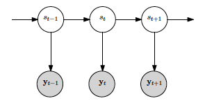
The Gaussian HMM manages the emission probabilities with gaussian distributions, its block diagram is represented in the next figure:

The parameters that we have to deal with are:

Where:

S is the hidden state sequence, being I the number of states of the model.
Y is the observed continuous sequence (in the discrete case, it would be the observed discrete sequence).
A is the matrix that contains the state transition probabilities.
B are the observation emission probabilities, which for the gaussian case are managed with the means and covariances.
π is the initial state probability distribution. In our model, both random and k-means can be used to initialize it.

Finally, the model's parameters of a HMM would be: θ={A, B, π}.

The three basic inference problems for HMMs

In order to have a useful HMM model for a real application, there are three basic problems that must be solved:

Problem 1: given the observed sequence Y, which is the probability of that observed sequence for our model's parameters θ, that is, which is p(Y | θ)?

To solve this first problem, the Forward algorithm can be used.

Problem 2: given the observed sequence Y and the model's parameters θ, which is the optimal state sequence S?

To solve this second problem several algorithms can be used, for example, the Viterbi or the Forward-Backward algorithm. If using Viterbi, we will maximize the p(S, Y | θ). Othercase, with the Forward-Backward algorithm, we optimizes the p(s_t, Y | θ).

Problem 3: which are the optimal θ that maximizes p(Y | θ)?

To solve this third problem we must consider the joint distribution of S and Y, that is:

By using the EM algorithm, the model parameters θ (that is, the initial state probability π, the state transition probabilities A and the gaussian emission probabilities {μ, Σ}) are updated.

The solution for these problems is nowadays very well known. If you want to get some extra knowledge about how the α, β, γ, δ... parameters are derived you can check the references below.

Heterogeneous HMM/HMM with labels

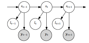
In the Heterogeneous HMM, we can manage some features' emission probabilities with discrete distributions (the labels) and some others' emission probabilities with gaussian distributions. Its block diagram is:

In addition to the parameters showed for the gaussian case, we must add:

Where:

L is the labels sequence.
D are the labels' emission probabilities.

For the Heterogenous HMM, our joint distribution is:

As we can observe in the previous equation, now the joint distribution depends on a new term which is the probability of the observed label given a certain state at an instant t.

Semi-Supervised HMM

The Semi-Supervised HMM is a version of the Heterogenous HMM where the label emission probabilities are set a priori. This allows us to asocciate certain states to certain values of the labels, which provides guidance during the learning process.

Missing Data Inference

Our model is able to work with both complete missing data and partial missing data. The first case is straight forward, and the mean of the state is used to compute the probability of the observation given a state and a time instant.

For the second case, that is, when we deal with partial missing data, we infer the value of the missed data. To do so, supposing x=(x_1, x_2) is jointly gaussian, with parameters:

The marginals are given by:

So the posterior conditional for our missing data can be obtained as:

References

Advanced Signal Processing Course, Prof. Dr. Antonio Artés-Rodríguez at Universidad Carlos III de Madrid
A tutorial on hidden Markov models and selected applications in speech recognition, L.R. Rabiner, in Proceedings of the IEEE, vol. 77, no. 2, pp. 257-286, Feb. 1989
Inference in Hidden Markov Models, O.Capp, E.Moulines, T.Ryden, Springer Publishing Company, Incorporated, 2010, ISBN:1441923195
Parallel Implementation of Baum-Welch Algorithm, M.V. Anikeev, O.B. Makarevich, Workshop on Computer Science and Information Technology CSIT'2006, Karlsruhe, Germany, 2006