This project implements Lucas-Kanade optical flow algorithm to track fluid motion patterns in video sequences. It's particularly useful for analyzing convection currents, eddy formations, and other fluid dynamic phenomena.
Click the image above to watch the demo video.
The script uses computer vision techniques to track the movement of points in a video sequence:
-
Grid Point Initialization:
- Creates a uniform grid of points across the video frame
- Points are spaced evenly in both x and y directions
- Default configuration uses a 10x10 grid (100 tracking points)
-
Lucas-Kanade Optical Flow:
- Implements the Lucas-Kanade method for optical flow calculation
- Tracks point movements between consecutive frames
- Uses pyramidal implementation for handling larger movements
- Key parameters:
- Window size: 15x15 pixels
- Pyramid levels: 2
- Termination criteria: 10 iterations or 0.03 epsilon
-
Trajectory Visualization:
- Each point is assigned a unique color
- Trajectories are drawn as continuous lines
- Real-time visualization of point movements
- Final output saved as MP4 video
The Lucas-Kanade method is based on three main assumptions:
- Brightness Constancy: The brightness of a pixel doesn't change between consecutive frames
- Temporal Persistence: The motion of a surface patch changes slowly in time
- Spatial Coherence: Neighboring points belong to the same surface and have similar motion
The algorithm solves the optical flow equation:
Ix*u + Iy*v = -It
where:
- Ix, Iy are image gradients
- It is temporal gradient
- u, v are the velocity components we want to compute
from optical_flow import track_grid_points

# Track points in video
trajectories = track_grid_points('path_to_video.mp4', grid_size=10)- OpenCV (cv2)
- NumPy
- Python 3.6+
pip install opencv-python numpyThe script generates:
- Real-time visualization window
- Output video file ('output.mp4') with tracked trajectories
- Trajectory data saved as CSV file ('trajectories.csv') for further analysis
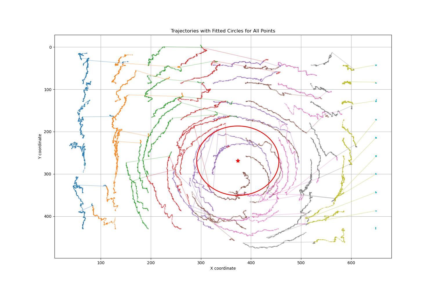
- Trajectory analysis visualization ('assets/trajectories_with_circles.png')
The project includes advanced trajectory analysis capabilities:
-
Data Processing:
- Trajectories are saved to CSV format with point IDs and coordinates
- Outlier removal using z-score thresholding
- Robust handling of incomplete or noisy trajectories
-
Circle Fitting:
- Fits circular paths to each point trajectory
- Uses least squares optimization to find best-fit circles
- Calculates center coordinates and radius for each trajectory
- Determines median circle parameters across all trajectories
-
Visualization:
- Plots all point trajectories with fitted circles
- Highlights median circle and center point
- Provides insights into overall fluid motion patterns
- Output saved as 'trajectories_with_circles.png'
MIT License
Feel free to open issues and pull requests for improvements!

