foxshakeitoff/dsc-interaction-terms-lab-v2-5

Interactions - Lab

Introduction

In this lab, you'll explore interactions in the Ames Housing dataset.

Objectives

You will be able to:

• Determine if an interaction term would be useful for a specific model or set of data
• Create interaction terms out of independent variables in linear regression
• Interpret coefficients of linear regression models that contain interaction terms

Ames Housing Data

Once again we will be using the Ames Housing dataset, where each record represents a home sale:

# Run this cell without changes
import pandas as pd

ames = pd.read_csv('ames.csv', index_col=0)

# Remove some outliers to make the analysis more intuitive
ames = ames[ames["GrLivArea"] < 3000]
ames = ames[ames["LotArea"] < 20_000]
ames

In particular, we'll use these numeric and categorical features:

# Run this cell without changes
numeric = ['LotArea', '1stFlrSF', 'GrLivArea']
categorical = ['KitchenQual', 'Neighborhood']

Build a Baseline Model

Initial Data Preparation

Use all of the numeric and categorical features described above. (We will call this the "baseline" model because we are making a comparison with and without an interaction term. In a complete modeling process you would start with a simpler baseline.)

One-hot encode the categorical features (dropping the first), and center (subtract the mean) from the numeric features.

# Your code here - prepare data for modeling

Build a Model with No Interaction Terms

Using the numeric and categorical features that you have prepared, as well as SalePrice as the target, build a StatsModels OLS model.

# Your code here - import relevant libraries and build model

Evaluate the Model without Interaction Terms

Describe the adjusted R-Squared as well as which coefficients are statistically significant. For now you can skip interpreting all of the coefficients.

# Your code here - evaluate the baseline model

# Your written answer here

Answer (click to reveal)

The model overall explains about 83% of the variance in sale price.

We'll used the standard alpha of 0.05 to evaluate statistical significance:

• Coefficients for the intercept as well as all continuous variables are statistically significant
• Coefficients for KitchenQual are statistically significant
• Coefficients for most values of Neighborhood are statistically significant, while some are not. In this context the reference category was Blmngtn, which means that neighborhoods with statistically significant coefficients differ significantly from Blmngtn whereas neighborhoods with coefficients that are not statistically significant do not differ significantly from Blmngtn

Identify Good Candidates for Interaction Terms

Numeric x Categorical Term

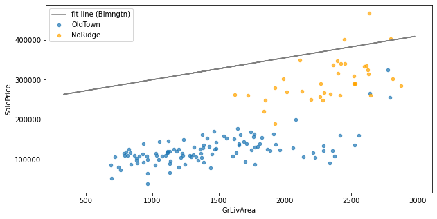
Square footage of a home is often worth different amounts depending on the neighborhood. So let's see if we can improve the model by building an interaction term between GrLivArea and one of the Neighborhood categories.

Because there are so many neighborhoods to consider, we'll narrow it down to 2 options: Neighborhood_OldTown or Neighborhood_NoRidge.

First, create a plot that has:

• GrLivArea on the x-axis
• SalePrice on the y-axis
• A scatter plot of homes in the OldTown and NoRidge neighborhoods, identified by color
  • Hint: you will want to call .scatter twice, once for each neighborhood
• A line showing the fit of GrLivArea vs. SalePrice for the reference neighborhood

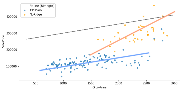
# Your code here - import plotting library and create visualization

Looking at this plot, do either of these neighborhoods seem to have a slope that differs notably from the best fit line? If so, this is an indicator that an interaction term might be useful.

Identify what, if any, interaction terms you would create based on this information.

# Your written answer here

Answer (click to reveal)

Your plot should look something like this:

If we drew the expected slopes based on the scatter plots, they would look something like this:

The slope of the orange line looks fairly different from the slope of the gray line, indicating that an interaction term for NoRidge might be useful.

Numeric x Numeric Term

Let's also investigate to see whether adding an interaction term between two of the numeric features would be helpful.

We'll specifically focus on interactions with LotArea. Does the value of an extra square foot of lot area change depending on the square footage of the home? Both 1stFlrSF and GrLivArea are related to home square footage, so we'll use those in our comparisons.

Create two side-by-side plots:

1. One scatter plot of LotArea vs. SalePrice where the color of the points is based on 1stFlrSF
2. One scatter plot of LotArea vs. SalePrice where the color of the points is based on GrLivArea

# Your code here - create two visualizations

Looking at these plots, does the slope between LotArea and SalePrice seem to differ based on the color of the point? If it does, that is an indicator that an interaction term might be helpful.

Describe your interpretation below:

# Your written answer here

Answer (click to reveal)

Your plots should look something like this:

For both 1stFlrSF and GrLivArea, it seems like a larger lot area doesn't matter very much for homes with less square footage. (In other words, the slope is closer to a flat line when the dots are lighter colored.) Then for homes with more square footage, a larger lot area seems to matter more for the sale price. (In other words, the slope is steeper when the dots are darker colored.)

This difference in slope based on color indicates that an interaction term for either/both of 1stFlrSF and GrLivArea with LotArea might be helpful.

For ease of model interpretation, it probably makes the most sense to create an interaction term between LotArea and 1stFlrSF, since we already have an interaction that uses GrLivArea.

Build and Interpret a Model with Interactions

Build a Second Model

Based on your analysis above, build a model based on the baseline model with one or more interaction terms added.

# Your code here - build a model with one or more interaction terms

Evaluate the Model with Interactions

Same as with the baseline model, describe the adjusted R-Squared and statistical significance of the coefficients.

# Your code here - evaluate the model with interactions

# Your written answer here

Answer (click to reveal)

The model overall still explains about 83% of the variance in sale price. The baseline explained 82.7% whereas this model explains 82.9%, so it's a marginal improvement.

• Coefficients for the intercept as well as all continuous variables are still statistically significant
• Coefficients for KitchenQual are still statistically significant
• Neighborhood_NoRidge used to be statistically significant but now it is not
• GrLivArea x Neighborhood_NoRidge is not statistically significant
• LotArea x 1stFlrSF is statistically significant

Interpret the Model Results

Interpret the coefficients for the intercept as well as the interactions and all variables used in the interactions. Make sure you only interpret the coefficients that were statistically significant!

# Your written answer here

Answer (click to reveal)

The intercept is about 258k. This means that a home with average continuous attributes and reference categorical attributes (excellent kitchen quality, Bloomington Heights neighborhood) would cost about \$258k.

The coefficient for LotArea is about 2.58. This means that for a home with average first floor square footage, each additional square foot of lot area is associated with an increase of about \$2.58 in sale price.

The coefficient for 1stFlrSF is about 30.5. This means that for a home with average lot area, each additional square foot of first floor area is associated with an increase of about \$30.50 in sale price.

The coefficient for LotArea x 1stFlrSF is about 0.003. This means that:

1. For each additional square foot of lot area, there is an increase of about \$2.58 + (0.003 x first floor square footage) in sale price
2. For each additional square foot of first floor square footage, there is an increase of about \$30.50 + (0.003 x lot area square footage) in sale price

Neighborhood_NoRidge and GrLivArea x Neighborhood_NoRidge were not statistically significant so we won't be interpreting their coefficients.

Summary

You should now understand how to include interaction effects in your model! As you can see, interactions that seem promising may or may not end up being statistically significant. This is why exploration and iteration are important!